Dispyr

Processing topographical data into monochromatic ink sketches.

This work is an attempt to emulate etching drawings with code, by playing with noise and data removal to create a natural rendering of random fragments of the Pyrénées.

𐫱

Inspiration and aims

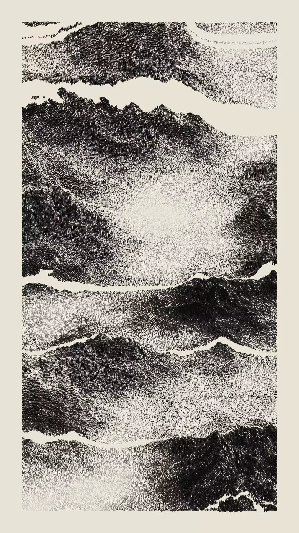
I was searching for an hybrid between the simplicity and efficiency of a famous data visualization in astronomy and the Meridian series by Matt Deslauriers. Moreover, to be able to use a pen-plotter to trace the images on paper, the algorithm should produce relatively long lines rather than the myriad of short segments that make Meridian appealing.

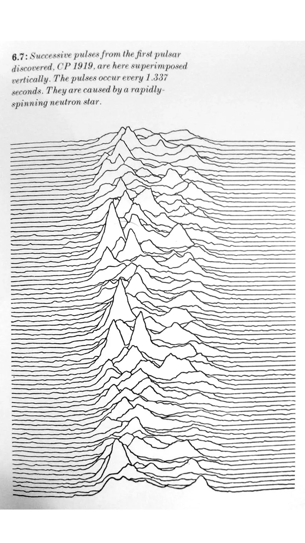
left : “Successive pulses from the first pulsar discovered, CP 1919, are here superimposed vertically. The pulses occur every 1.337 seconds. They are caused by rapidly spinning neutron star.” From The Cambridge Encyclopaedia of Astronomy.
right : Meridian #638

This algorithm feeds on elevation data produced by public structures with different technologies (image analysis, topographical radar, or lidar) and made available for reuse. In this sense, it differs from generative art, where the code is self-sufficient to produce results (see why-love-generative-art) This short article explains the underlying logic and software code. A basic reproducible example is available here to encourage creative experiments.

I won’t comment much on the choice of the R language and the code itself. It’s just that I knew this language for work, and I was curious to see if i could reuse it for other projects. For me, the functional programming paradigm makes sense to interact with code, moreover when working in interrupted streaks. The broad data exploration workflow resonate with my somewhat reductionist creative approach, especially how the tools for data visualization enable to focus on visual experiments rather code for graphics. I also went for the easy way, thanks to the creators of incredible libraries for (spatial) data processing and graphics. For this project I used {{stars}}, {{dplyr}}, and {{ggplot2}}.

The algorithm is composed by three main functions, created to be used successively (with the R pipe function, |>). This article broadly illustrates the content of these functions.

get_features_ridge(seed = 15) |> gen_dispyr(n_ridges = 800) |> plot_ridge()

1. get_features_ridge() is a function of a random seed, and is used to generate the main features of the output (e.g. the location, orientation, style)
2. gen_dispyr() uses this set of features to download and process data from a digital elevation model (3D) into a set of lines (2D).
3. plot_ridge() renders the processed data into a vector image.

Process

Features generation

The outputs have only two broad features: a random location in the Pyrénées mountain range and a rendering style, randomly chosen among four methods with a set of probabilities. Most of the visual variability in the outputs is driven by the choice of geographical location, it gives the series a strong link with the subject, but somehow limits the maximum number of obtainable iterations.

Location

To get a random location in the Pyrénées mountain range, we first define a sampling region (a 20 km wide buffer around the French-Spain border), and use sf::st_sample to sample a location in this polygon. The code is simplified to sample a mysterious location in a polygon defined by the Andorra borders.

# load a polygon of the Andorra borders
polygon <- rnaturalearth::ne_countries(
  country = c("andorra"), scale = "medium", returnclass = "sf"
  ) |> st_transform(2154)

# get a sample in the defined polygon 
coord <- st_sample(polygon, size = 1) |> st_as_sf()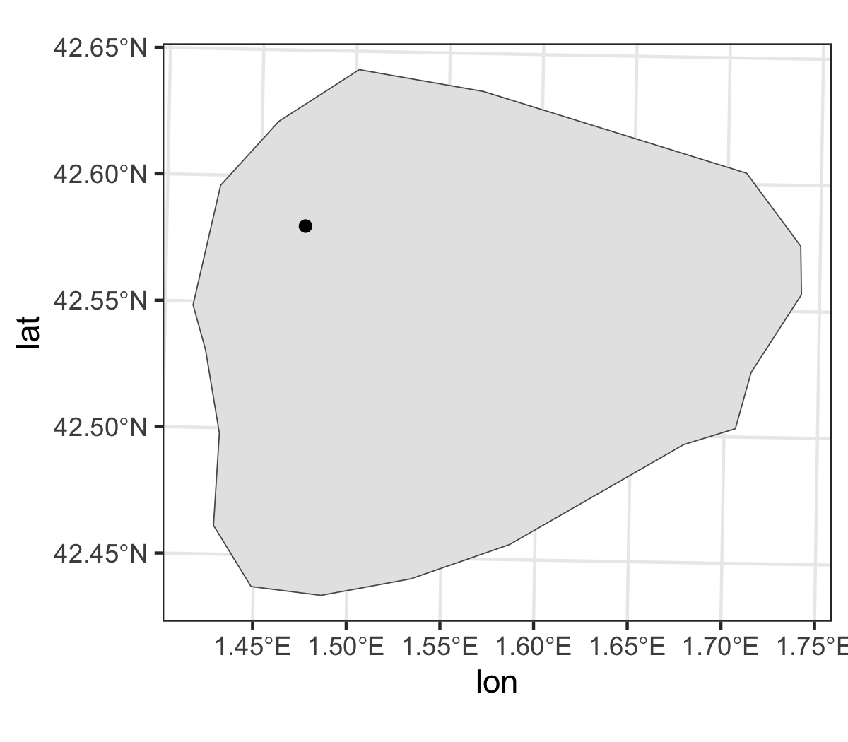

Rendering style

The overall rendering style is impacted by a dozen parameters in the code (e.g. line density, position of lines in the y-axis, amount and position of removed data). Rather than a free exploration of this parameter space, which could lead to heterogeneous outputs, I defined a limited number of fixed sets of parameters. I created four styles, and named them as weather conditions (clear, mist, snow, storm).

Technically nothing complicated, the get_features_ridge() function returns a list of features and associated parameters, later used for the data processing step. The parameters are presented at the moment they are used in the code.

Data processing

This stage uses the previous set of features to download and process data from a digital elevation model (3D) into a set of lines (2D), with distinct processing steps.

Getting a realistic description of the landscape

This step start by actually retrieving the elevation data around the sampled location (a 2x2 km square for the illustration, 20x15 km normally). The {{elevatr}} R package makes this step a breeze, but the process is the same when using local high-resolution data.

# get DEM data in a 2x2 km region around the sampled point
dem <- elevatr::get_elev_raster(
  coord, z = 11, expand = 1E3, clip = "bbox") 

# use a heatmap to glance at elevation data
plot <- ggplot() +
  geom_stars(data = st_as_stars(dem)) +
  geom_sf(data = coord, color = "white", size = 1) +
  scale_fill_viridis_c(name = "elevation") +
  labs(x = "lon", y = "lat")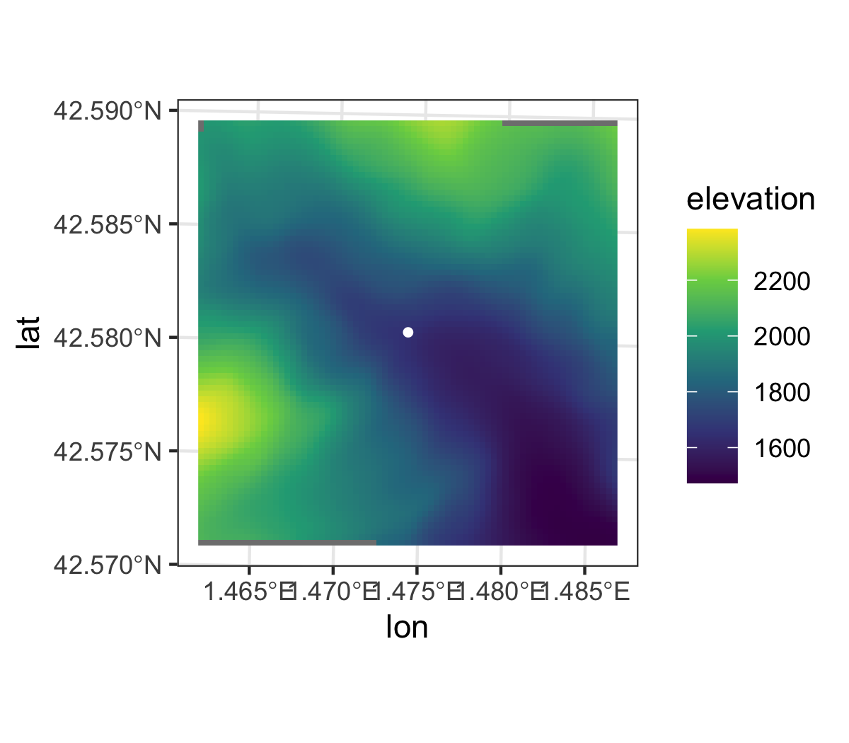 

Slicing the landscape into lines

The aim is to process a 3D point set into 2D lines, by computing multiple lines of elevation as a function of longitude, for discrete latitude values. This step is perfectly illustrated by the stacked plot of radio signals presented previously. In our case, each line corresponds to one row in the elevation data (74x74 matrix in the example). Without further modifications, the output is unclear, with a lot of intersecting lines (figure A).

To improve the output readability, but also introduce potential for variations, we process this raw elevation matrix with two actions:

• shift lines in the y-direction as a function of their rank from the foreground.
• delete the line segments that should be hidden by foreground lines with a higher elevation.

# parameters
z_shift = 5

# convert DEM from spatial to dataframe format
df_dem <- dem |> stars::st_as_stars() |>
  as_tibble() |> select(x, y, z = 3)  

# compute elevation shift as a function of normalized distance
data_index <- df_dem |>
  distinct(y) |> arrange(y) |>
  mutate(
    y_rank = rank(y),
    y_dist = scales::rescale(y, to = c(0,1)),
  ) |>
  mutate(dz = y_rank * z_shift)

# compute shifted elevation values
df_shift <- df_dem |> 
  left_join(data_index, by = "y") |>
  group_by(y) |> mutate(xn = x - min(x), x_rank = rank(x)) |> ungroup() |>
  mutate(zs = z + dz)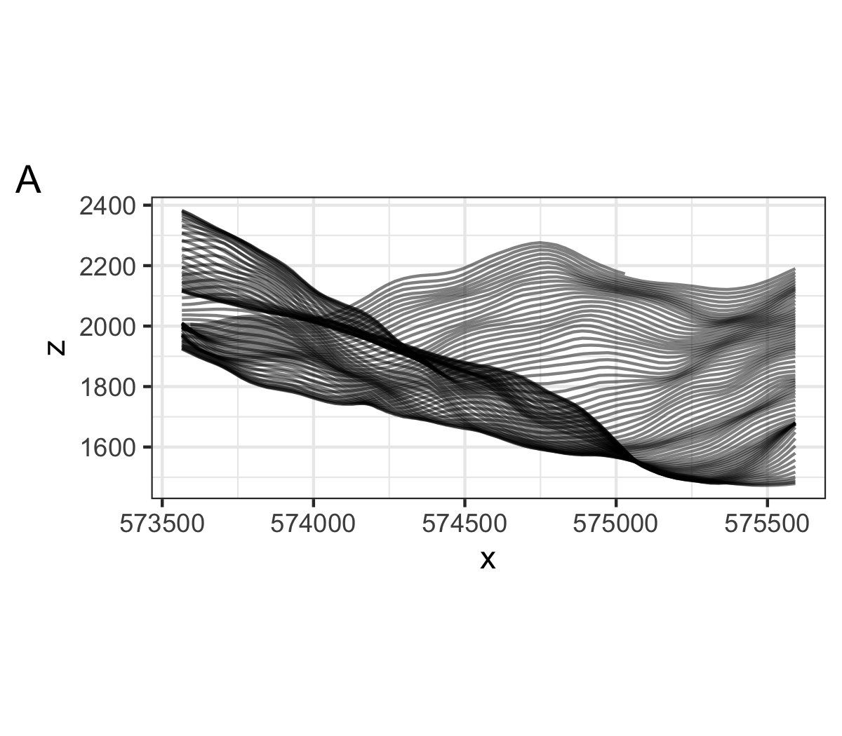

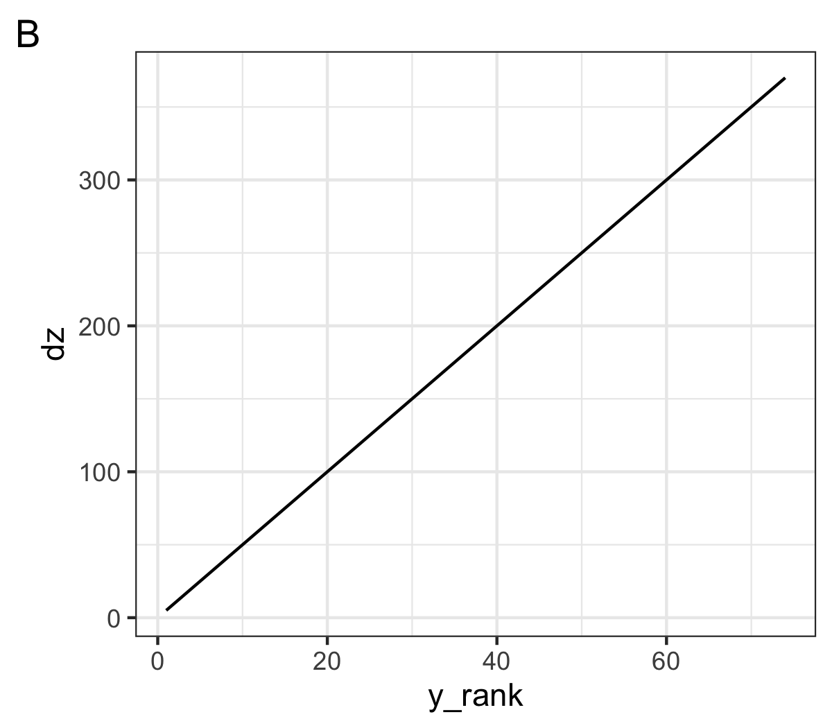
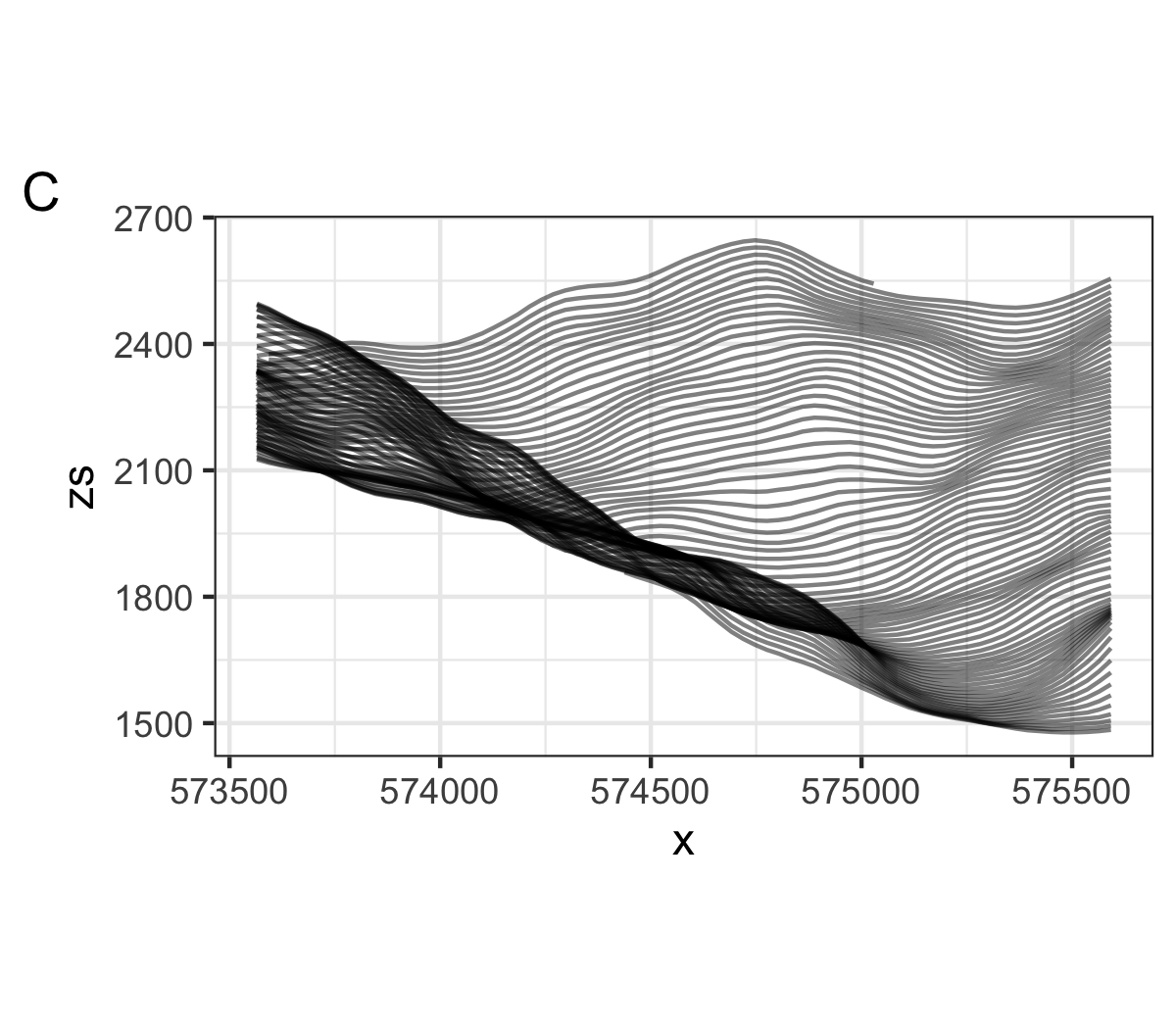
The shifting step calculates the difference from the reference elevation as a linear function of its rank from the foreground (figure B). Increasing the slope of this function impacts the perspective, towards a more aerial view of the landscape, eventually reducing the number of intersecting lines (figure C). Using non-linear functions creates unrealistic but interesting perspectives.

At this step, a fast solution to achieve line intersection is by drawing lines with a filled area underneath, starting from the background and thus progressively masking previous polygons (as in painter’s algorithm). This solution is implemented directly in the ggridges R package. But this option is not ideal for creative coding : the hidden lines still exist, which makes vector outputs unusable with a pen-plotter, and it lacks flexibility on the overlaying method.

# parameters
n_lag = 100
z_threshold = 0

# define window functions for multiple lag positions
list_distance <- map(glue::glue("~ . - lag(., n = {1:n_lag})"), ~ as.formula(.))
list_col <- glue::glue("zs_{1:n_lag}")

# remove points hidden by foreground ridges :
# compute lagged elevation difference between successive y for each x 
# replace value by NA when the difference is less than a threshold 
df_ridge <- df_shift |> 
  arrange(y_rank) |> group_by(x) |>
  mutate(across(zs, .fns = list_distance)) |>
  ungroup() |> 
  mutate(
    zn = case_when(
      if_any(all_of(list_col), ~ . < z_threshold) ~ NA_real_,
      TRUE ~ zs)) |>
  select(- all_of(list_col))

In the code above, the intersections between lines are avoided by checking for a minimum distance between a point at a given x position and its neighbourhood along y, and removing the point if any points in the neighbourhood falls below this distance (z_threshold parameter). To avoid computing the distance matrix for all points (74⁴, in this small area), we only check for intersections along a limited range (n_lag parameter, between 0 and 300 y ranks). Increasing the threshold parameter creates clearer distinction between the sides of mountains.

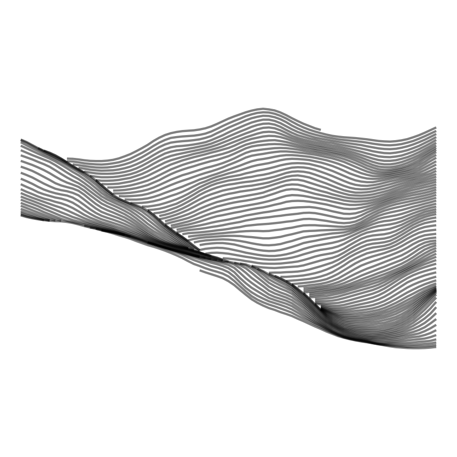
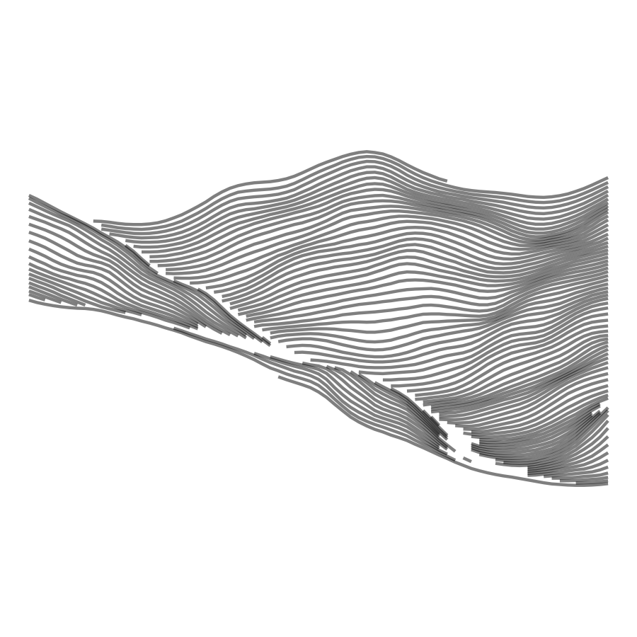
Line segments are hidden by foreground lines by using polygon masking (left) or distance-based point removal with a null (center) or positive threshold (right).

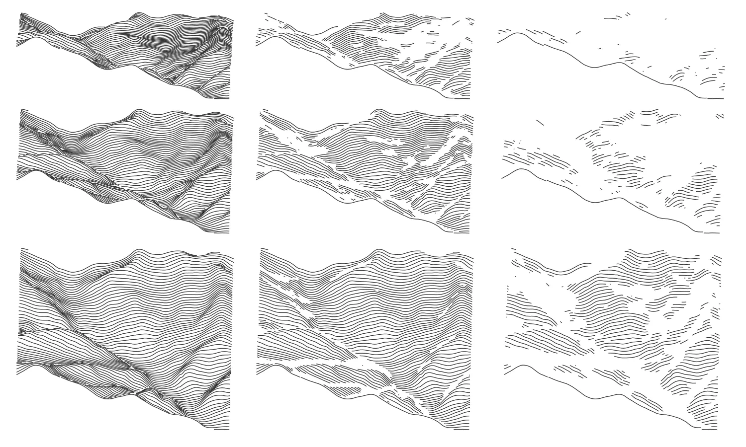
Effect of shift (in rows) and threshold (in columns) parameter combination on the landscape rendering (16 km²).

Altering the lines with noise and deletion

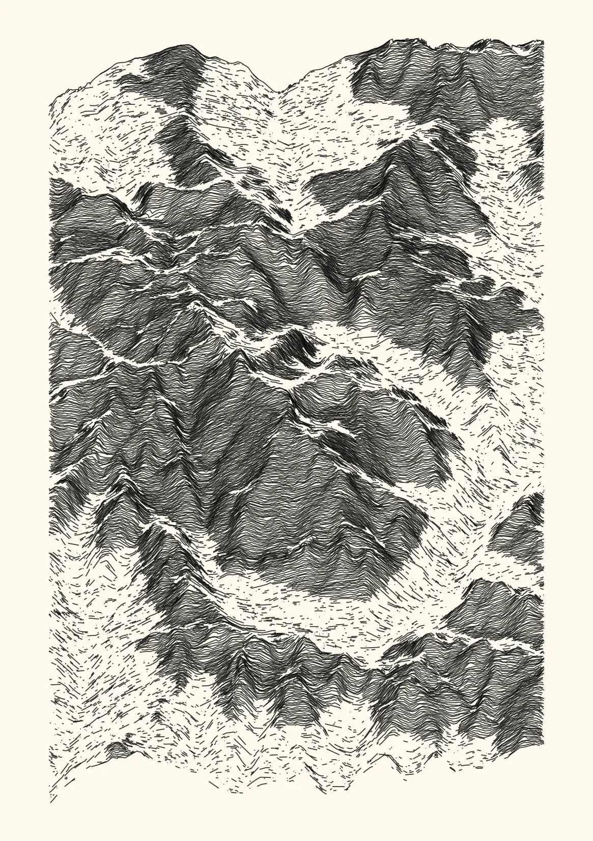
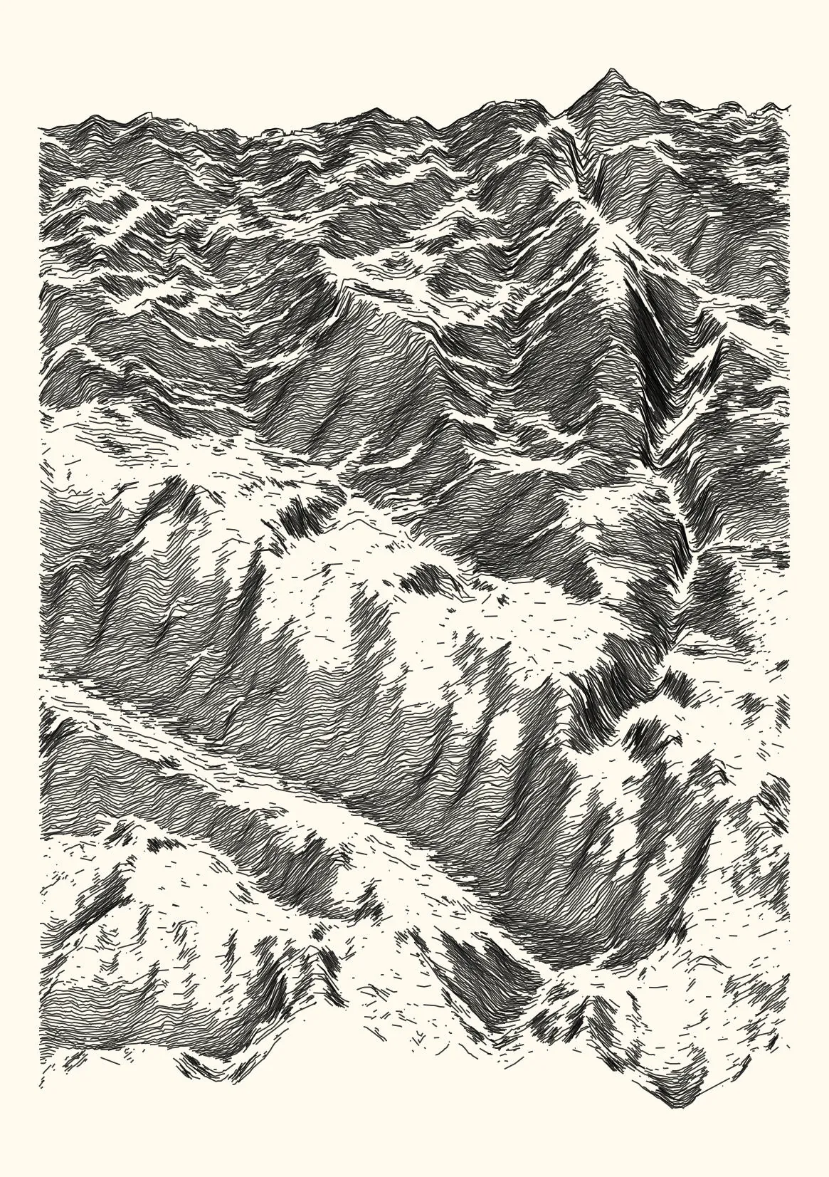
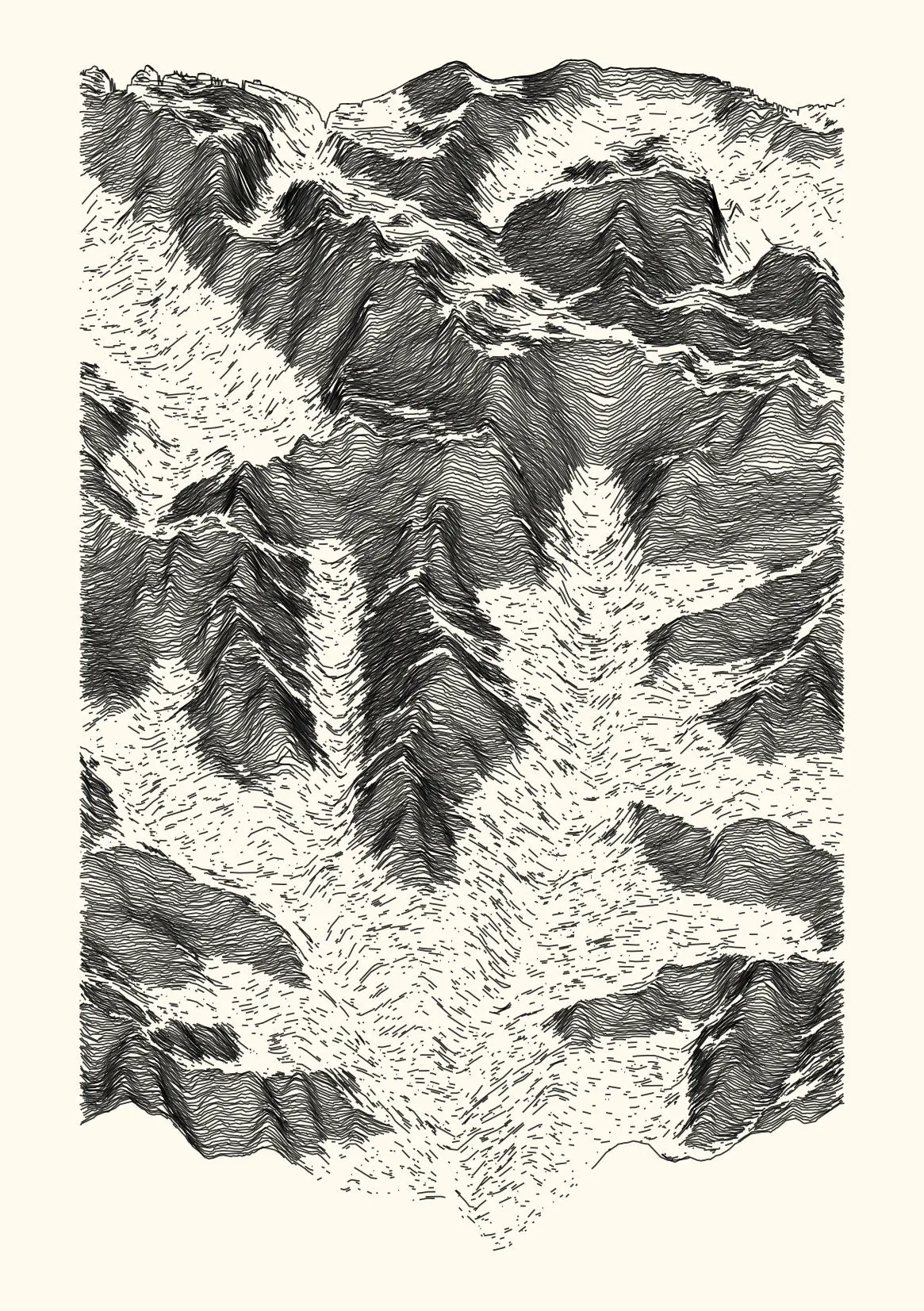
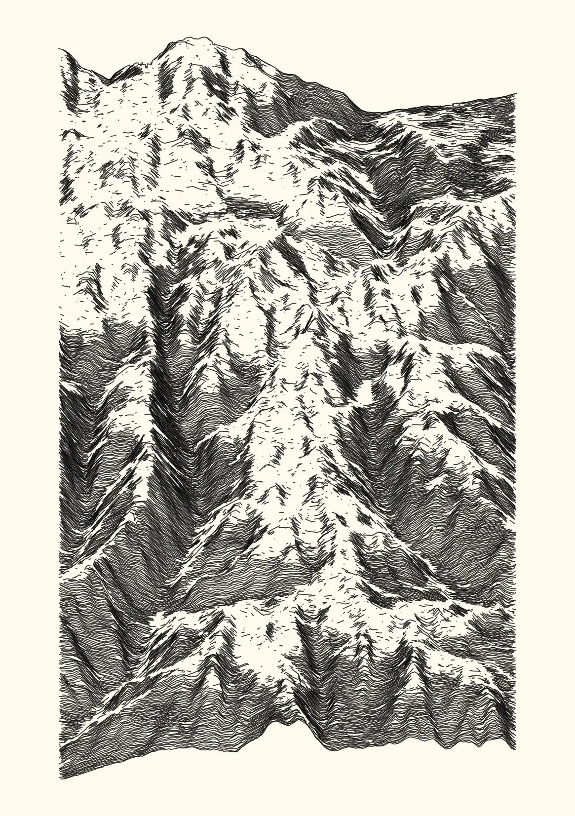
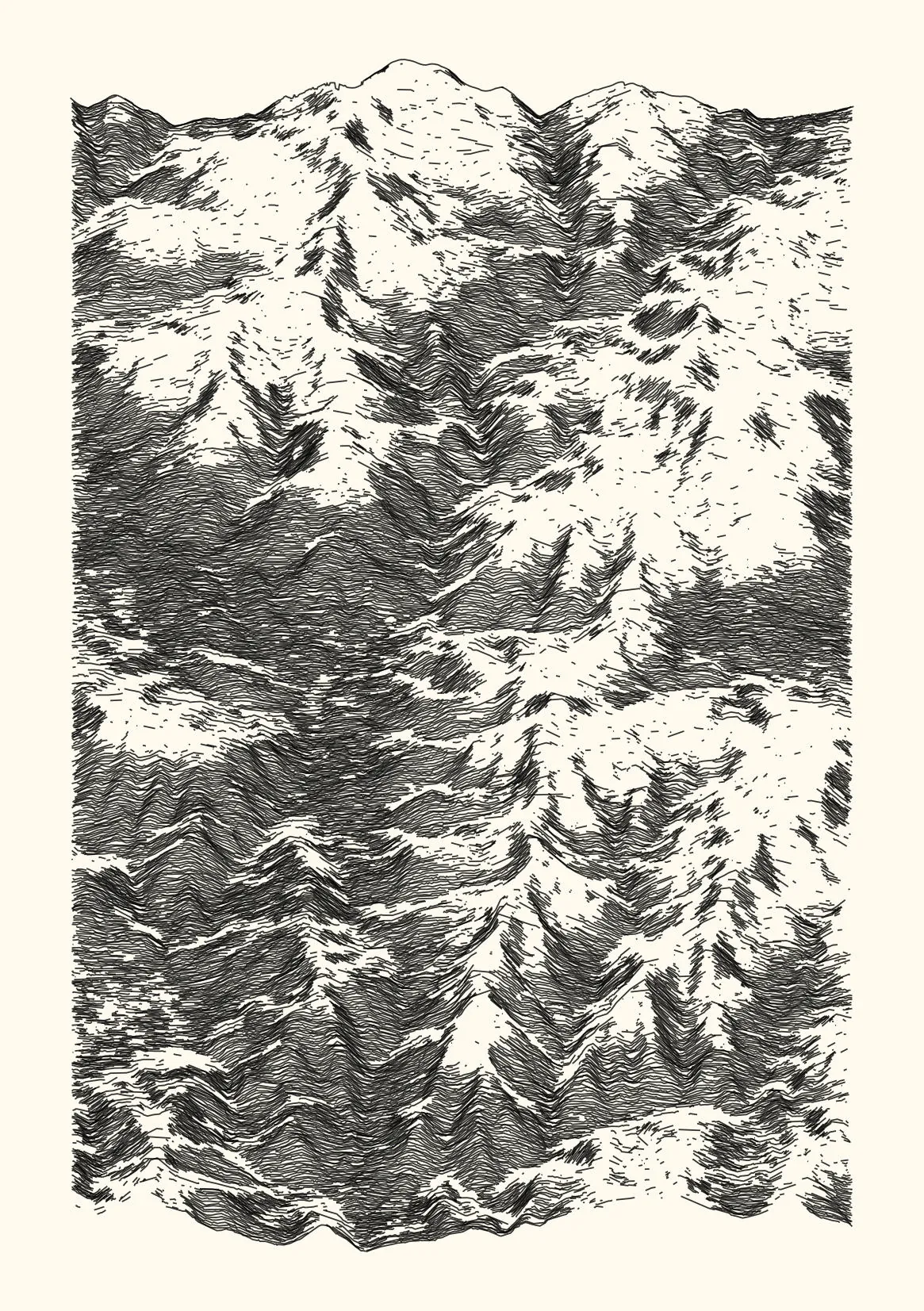
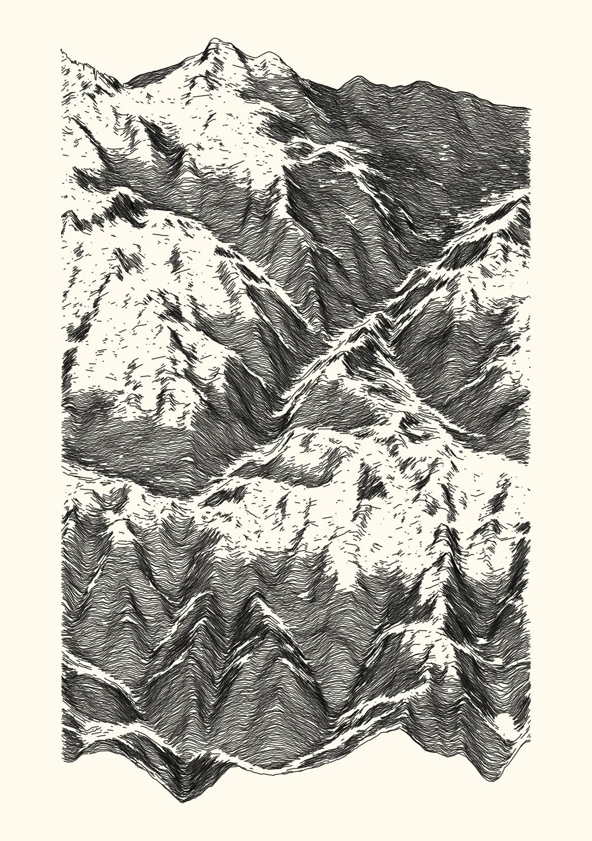
Finally, the overall aesthetic is obtained by adding noise and discarding data as a function of various attributes (elevation, slope, elevation dispersion). The governing idea was to test how our perception of the landscape changes when most of the initial topographical data is perturbed or removed. Here are four methods, but much is left to explore. The illustration code here is functioning without external call, but highly redundant and surely not optimal, you can conveniently hide it if you feel horrified.

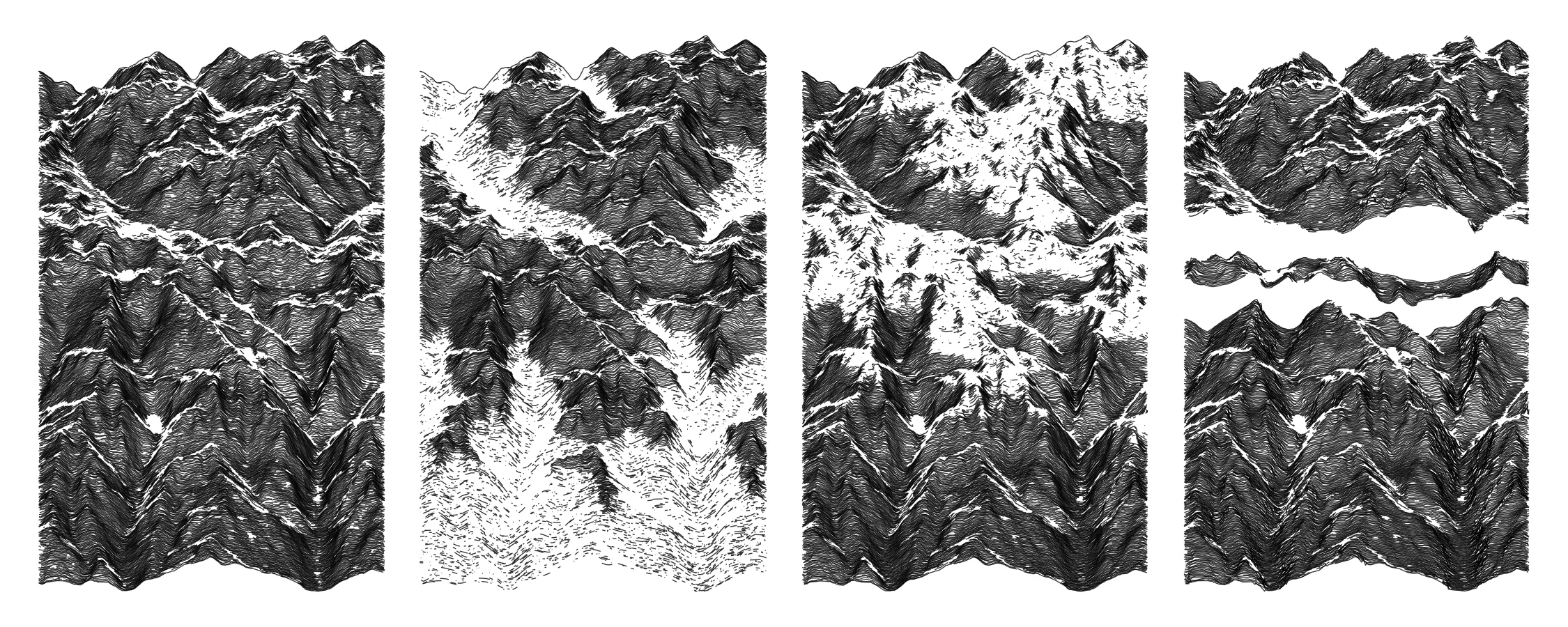
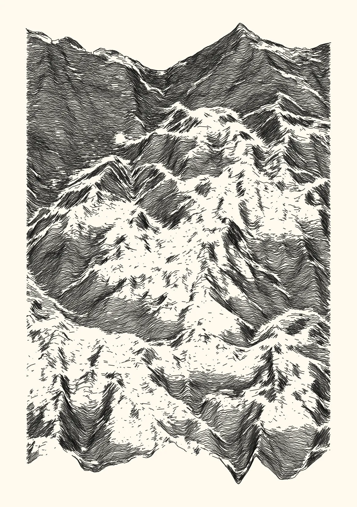
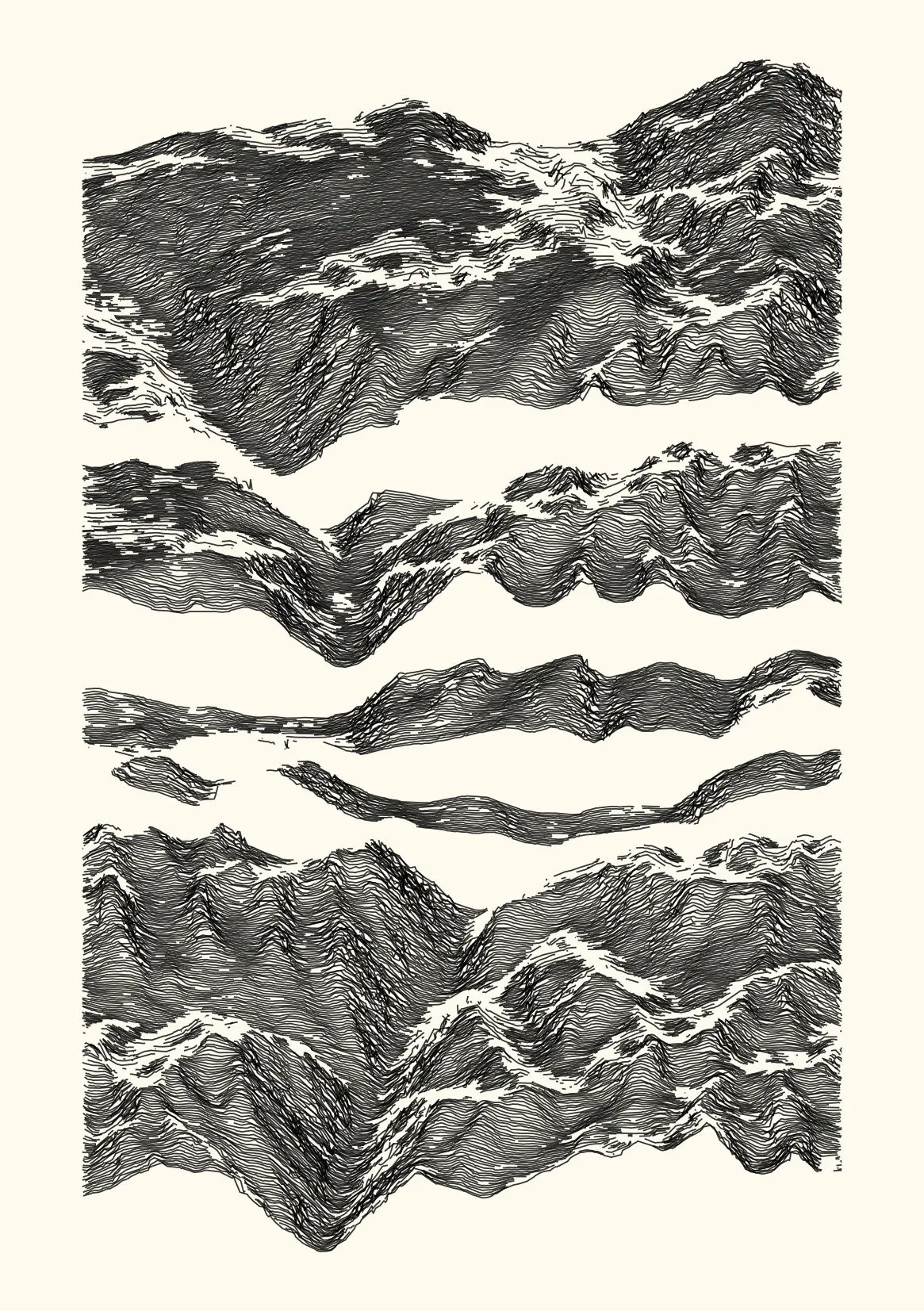
Four data processing methods, all based on filtering points and adding noise, and named after weather conditions (clear, mist, snow, storm).

clear

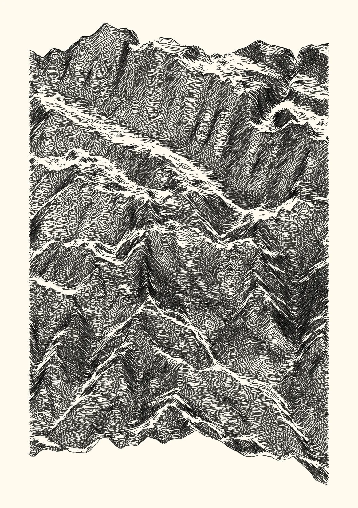
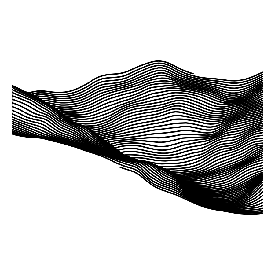
For each ridgeline, the method samples 50 % of the points and adds moderate jitter on elevation values.

# parameters
z_remove = 0.5      # proportion of points to remove
z_jitter = 4        # amount of jitter in elevation values

# randomly sample a proportion of points in a line, jitter their y-position.
df_plot <- df_ridge |>
  group_by(y_rank) |>
  slice_sample(prop = (1 - z_remove)) |>
  mutate(zn = jitter(zn, amount = z_jitter))

# plot output
df_plot |> ggplot(aes(x, zn, group = y)) +
  geom_line(alpha = 0.5) + coord_fixed() + theme_void() 

mist

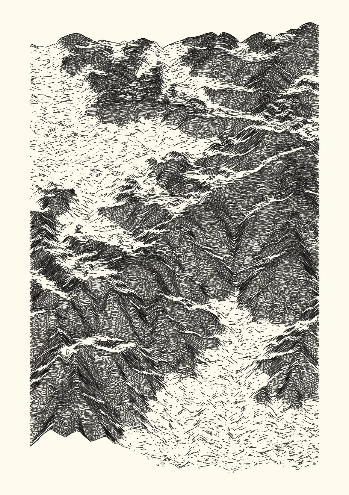
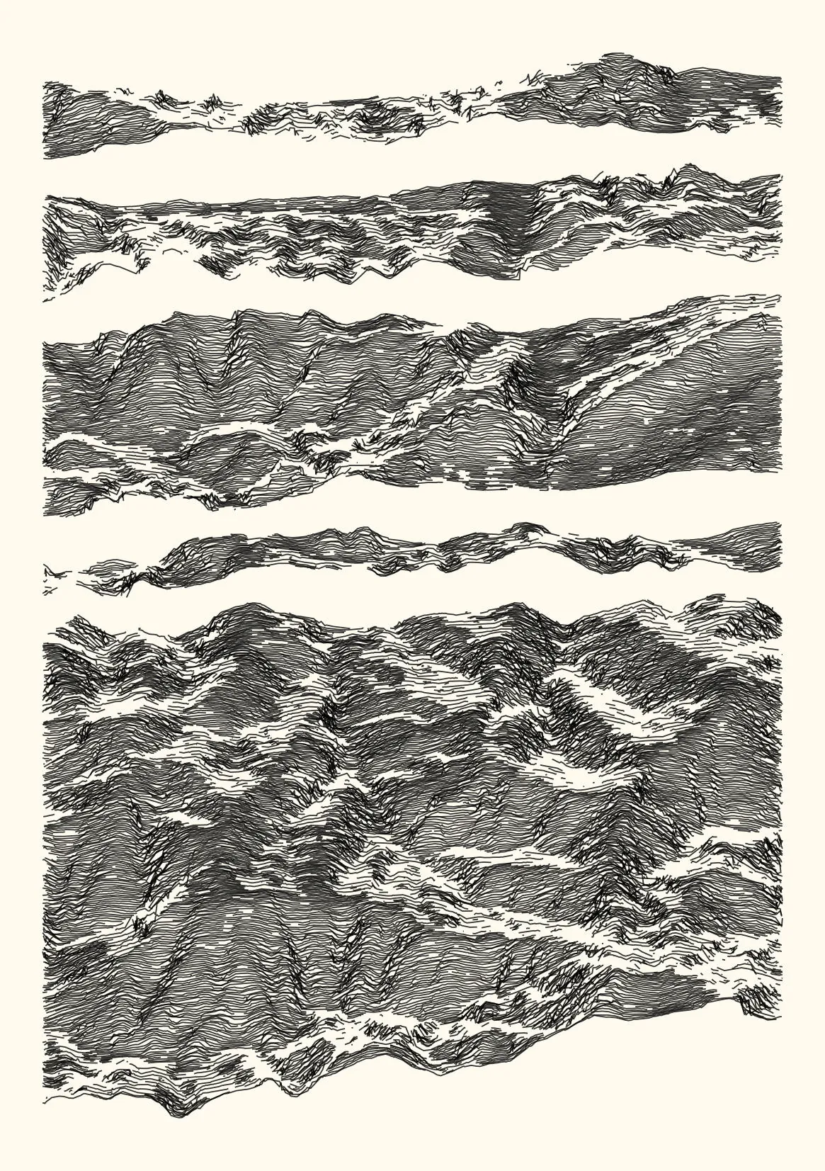
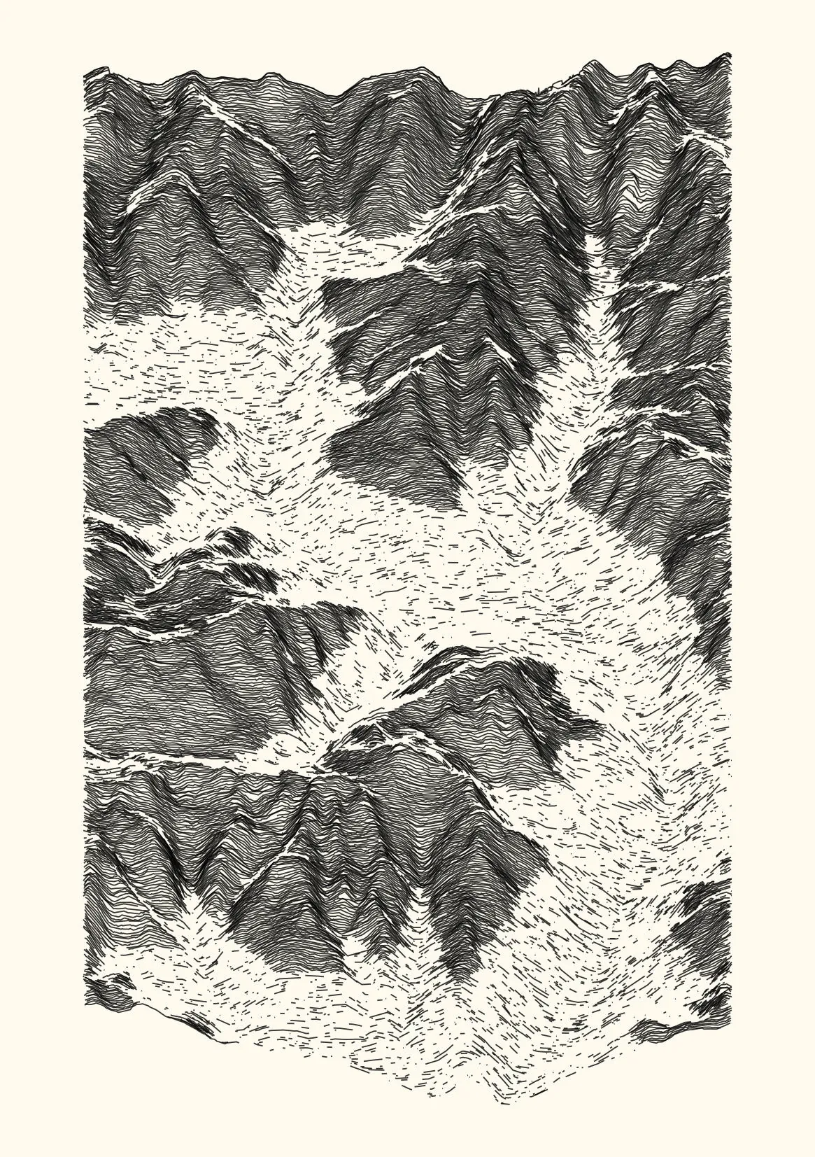
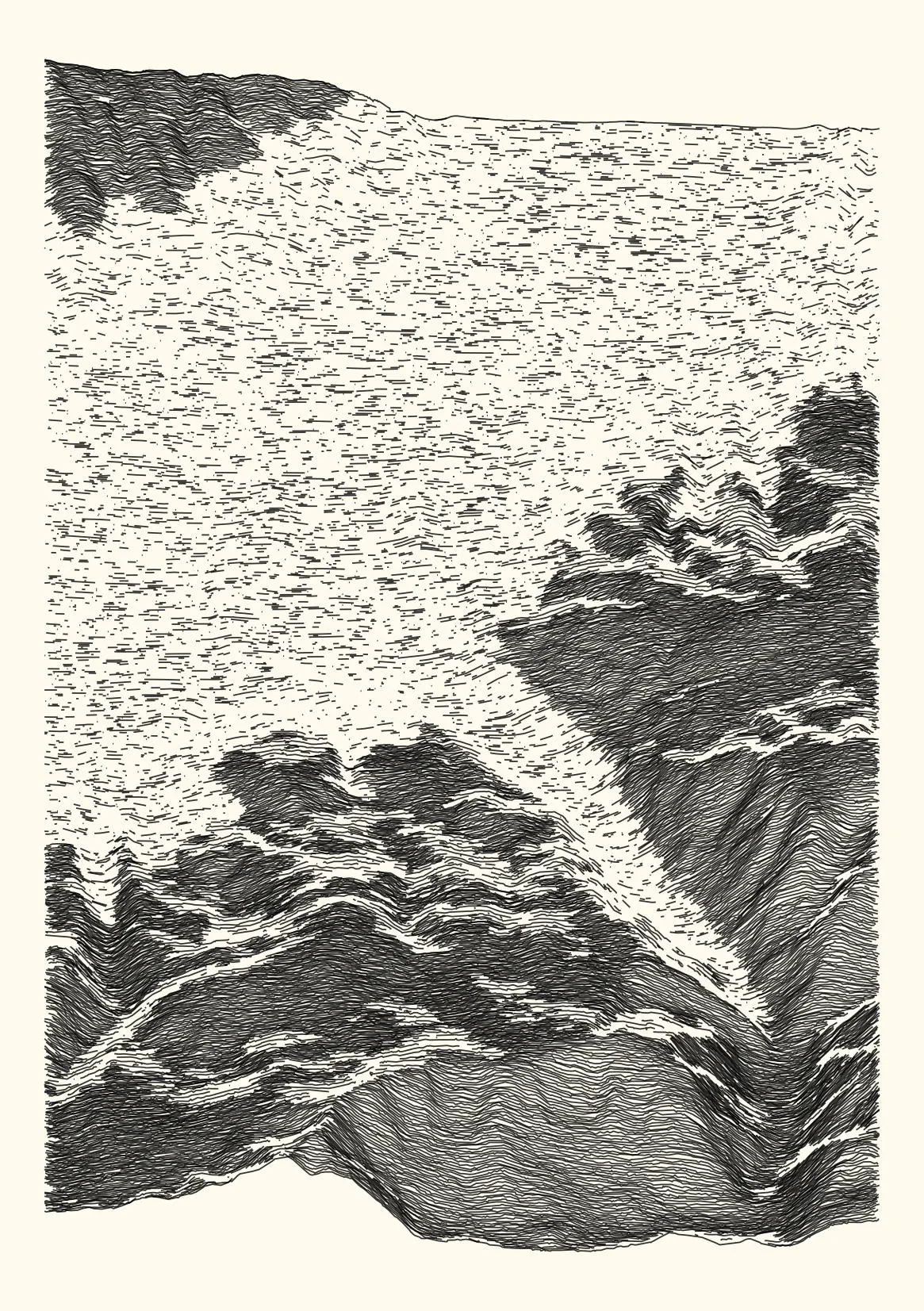
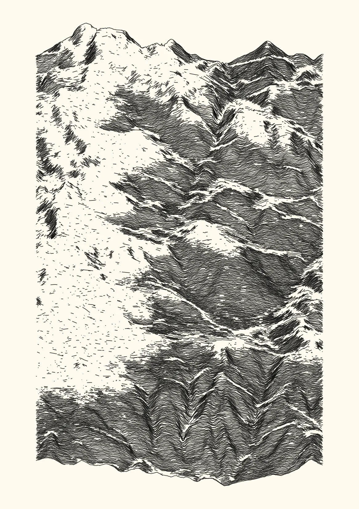
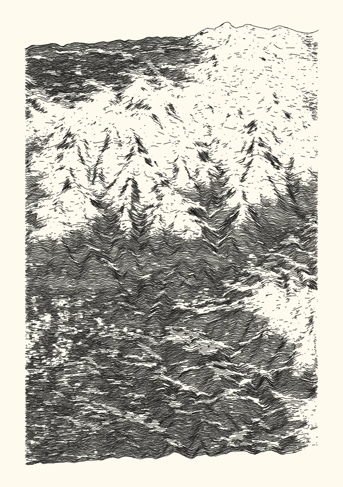
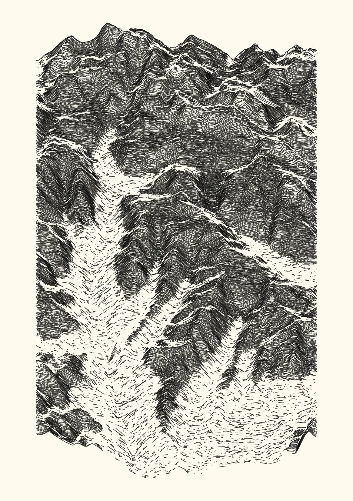
Same base as the previous method. In addition, when below an elevation threshold, lines are smoothed and points are randomly removed.

# functions

# add a proportion of missing values in a vector
sample_missing <- function(x, p) {
  n <- length(x)
  s <- sample(1:n, size = p * n)
  x[s] <- NA
  return(x)
}

# parameters
x_size = 10         # window of the rolling average 
z_limit = 0.5       # quantile value determining the elevation threshold
z_remove = 0.5      # proportion of points to remove in lines
z_missing = 0.2     # proportion of missing value to add
z_jitter = 4        # amount of jitter in elevation values

# calculate elevation cut
z_cut = quantile(df_ridge$z, z_limit, na.rm = TRUE)

# smooth lines with a rolling mean 
df_smooth <- df_ridge |>
  group_by(y_rank) |>
  mutate(
    zm = RcppRoll::roll_mean(zn, n = x_size, fill = NA),
    zm = case_when(
      (is.na(zm) & (x_rank < x_size/2 | x_rank > max(x_rank) - x_size/2)) ~ zn,
      TRUE ~ zm)) 

# remove data as a function of elevation, jitter y-position above a threshold   
df_plot <- df_smooth |> 
  slice_sample(prop = (1 - z_remove)) |>
  mutate(
    zn = case_when(
      (z < (z_cut - 200)) ~ sample_missing(zm, p = z_missing + 0.2),
      (z < z_cut)         ~ sample_missing(zm, p = z_missing),
      TRUE                ~ zn),
    zn = if_else(z > z_cut, jitter(zn, amount = z_jitter), zn)
  ) 

# plot output
df_plot |> ggplot(aes(x, zn, group = y)) +
  geom_line(alpha = 0.5) + coord_fixed() + theme_void()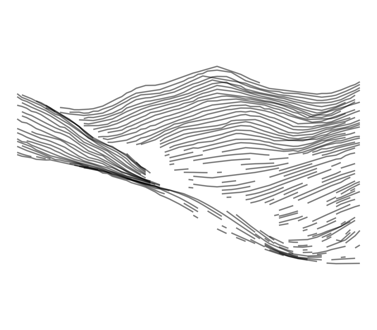 

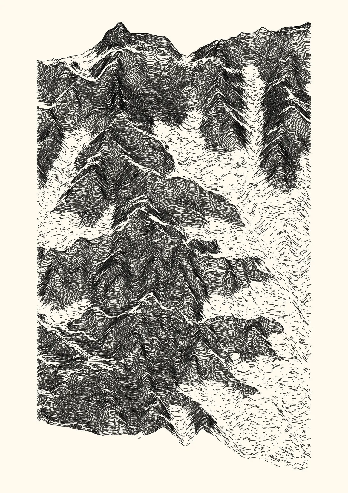
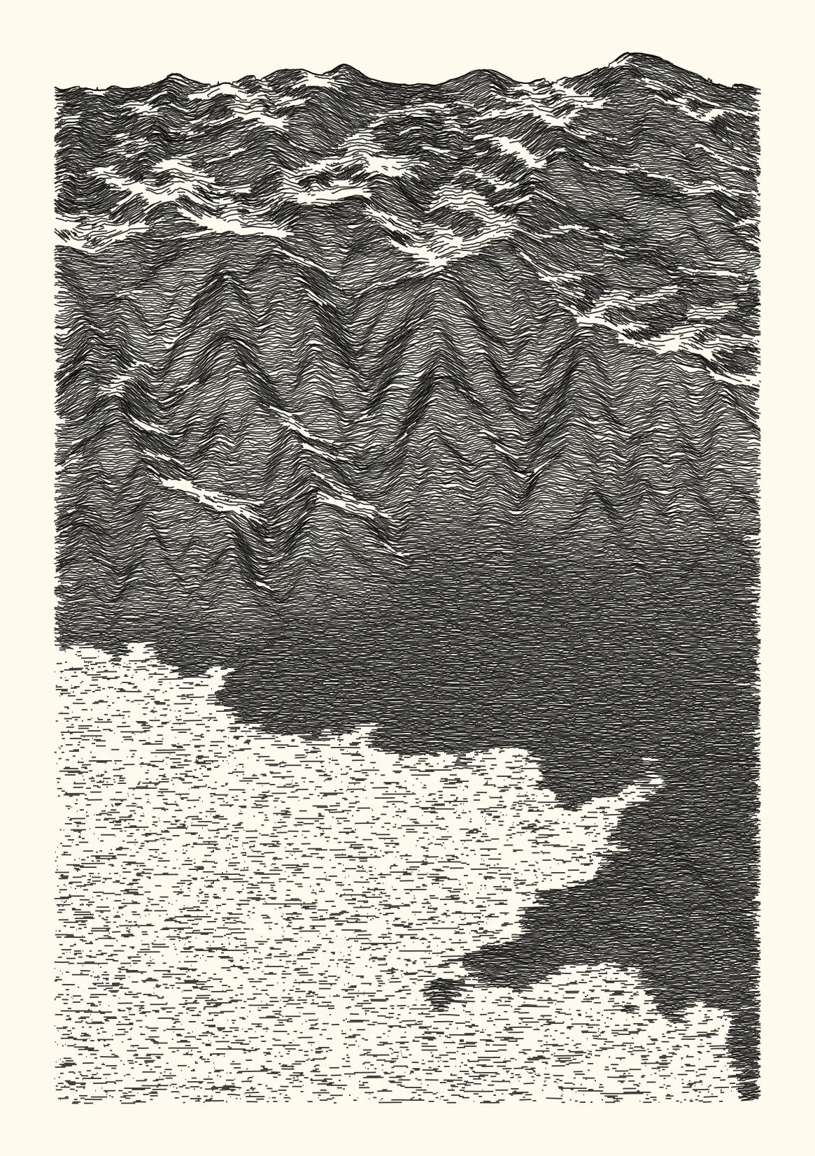
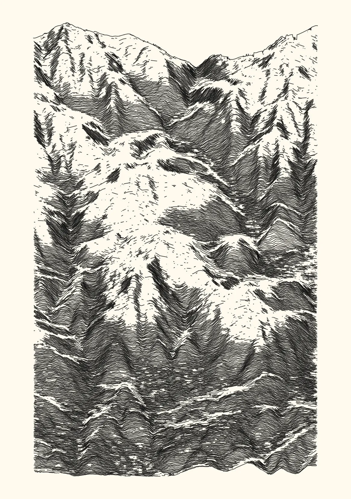
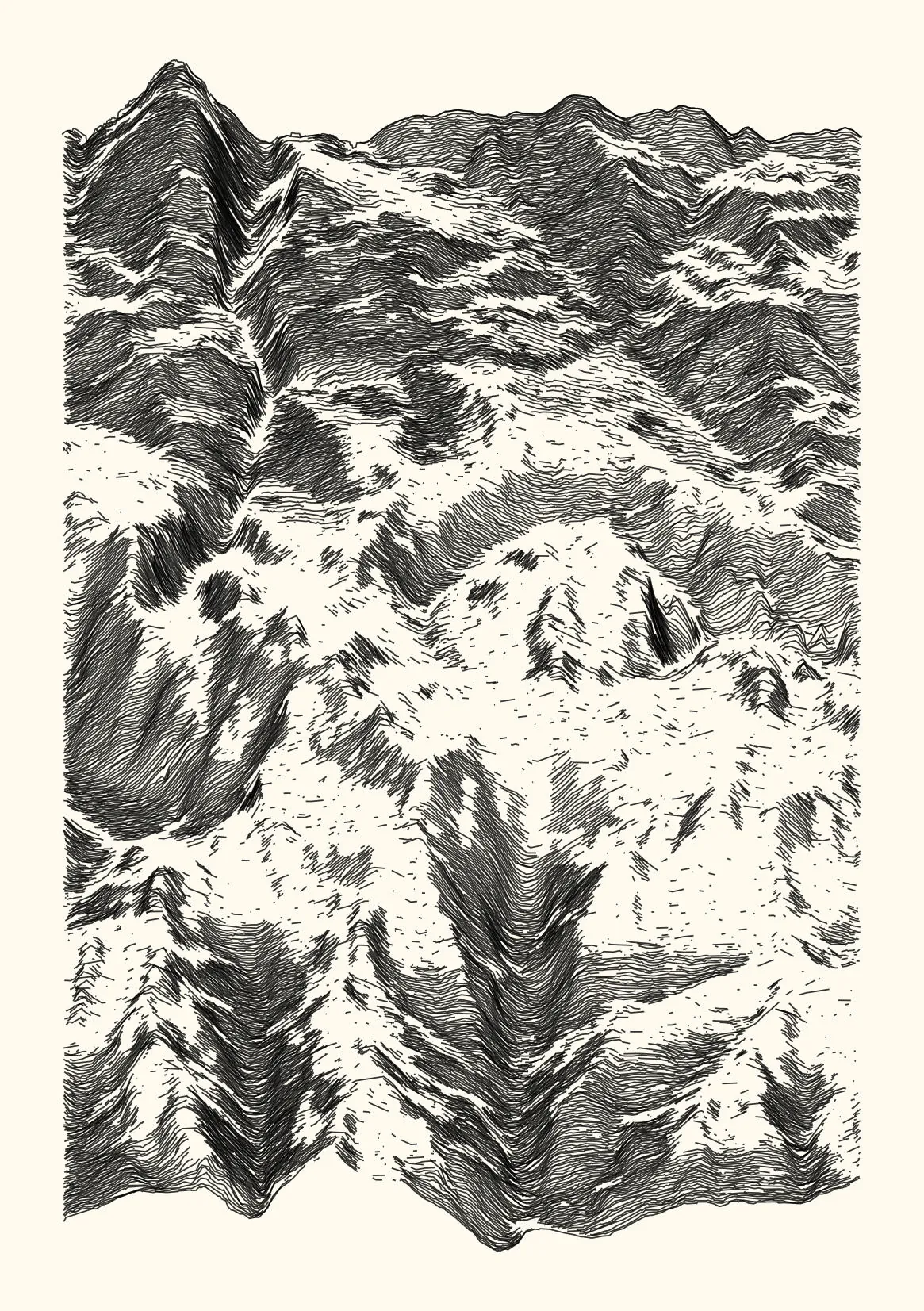
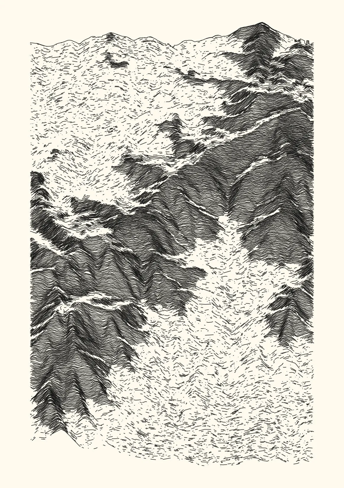
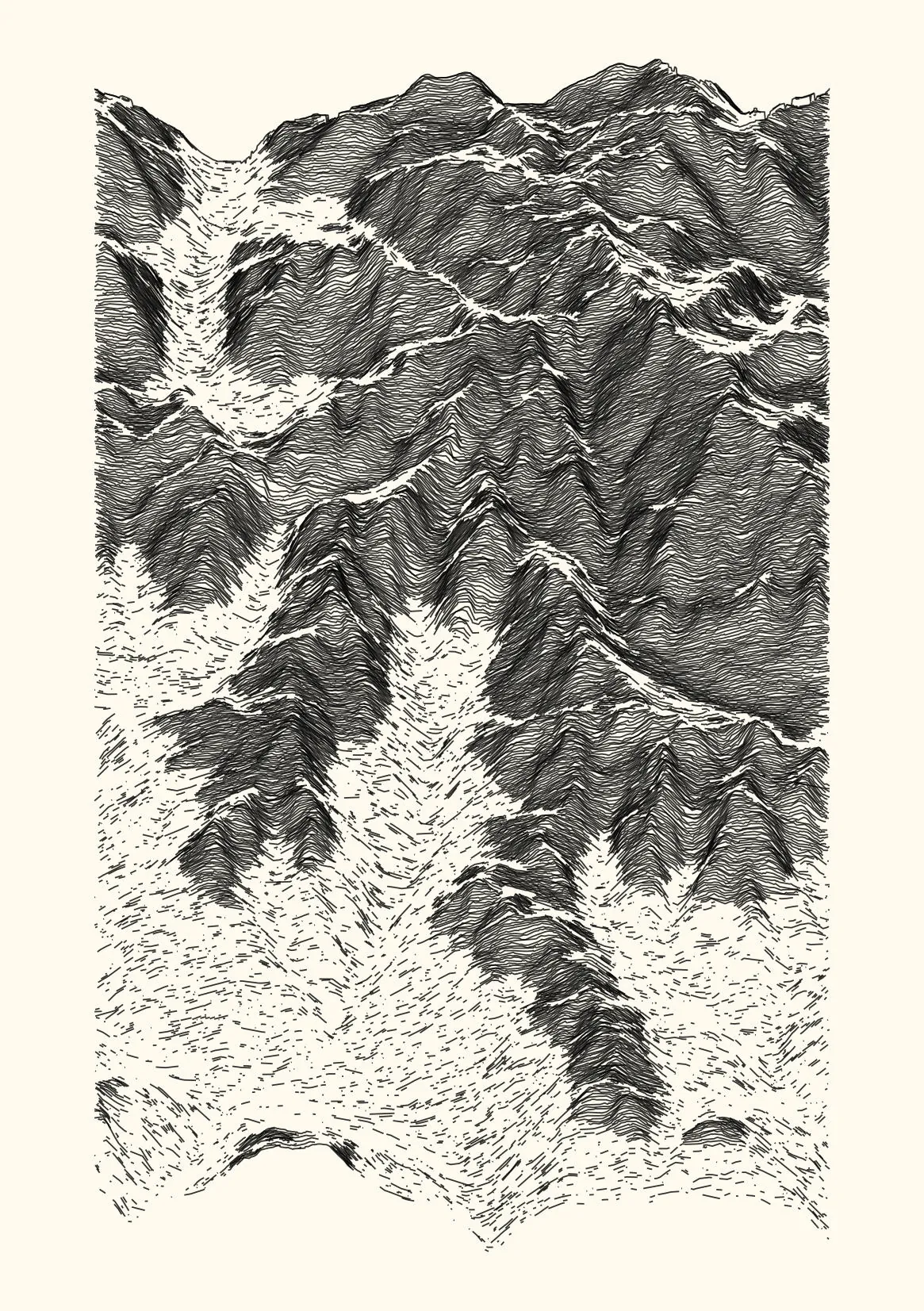
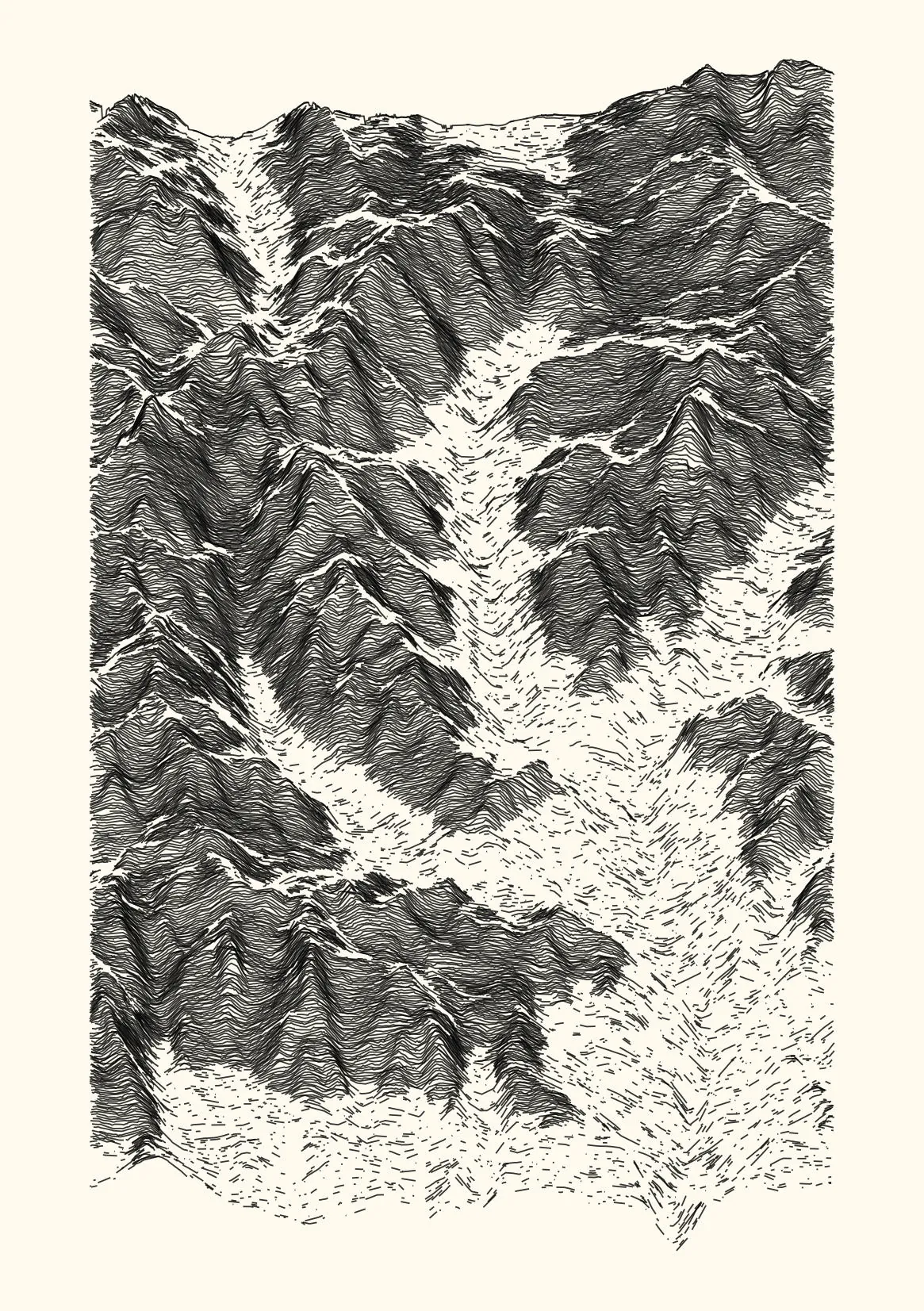
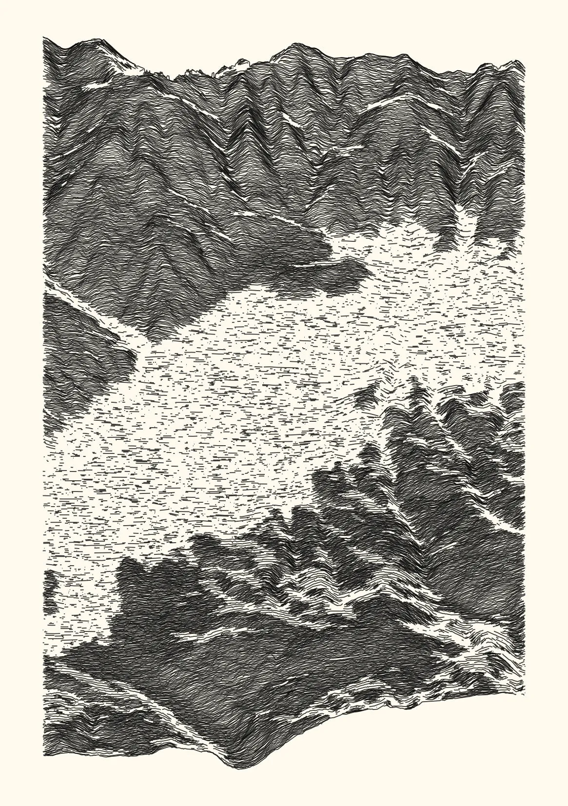
snow

Same base as the previous method, but the data removal is also a function of a slope threshold.

# parameters
x_size = 5          # window of the rolling average 
z_limit = 0.7       # quantile value determining the elevation threshold
z_remove = 0.5      # proportion of points to remove in lines
z_missing = 0.6     # proportion of missing value to add
z_jitter = 4        # amount of jitter in elevation values

# calculate elevation cut
z_cut = quantile(df_ridge$z, z_limit, na.rm = TRUE)

# calculate local slope and remove points for flat areas
df_filter <- df_ridge |>
    group_by(y_rank) |> arrange(x_rank) |>
    mutate(
      z_slope = abs(
        (zn - lag(zn, default = 0)) / (xn - lag(xn, default = 0))
        ),
      z_slope = RcppRoll::roll_mean(z_slope, n = x_size, fill = NA_real_),
      zn = if_else(z_slope == 0, NA_real_, zn)
    ) |> ungroup()

# remove data as a function of slope and elevation   
df_plot <- df_filter |>
  group_by(y_rank) |>
  slice_sample(prop = (1 - z_remove)) |>
  mutate(
    zn = case_when(
      (z > z_cut) & (z_slope < 60/100)         ~
        sample_missing(zn, p = z_missing),
      (z > (z_cut - 100)) & (z_slope < 60/100) ~
        sample_missing(zn, p = z_missing / 2),
      TRUE                                     ~
        zn),
    zn = jitter(zn, amount = z_jitter)
  ) 

# plot output
df_plot |> ggplot(aes(x, zn, group = y)) +
  geom_line(alpha = 0.5) + coord_fixed() + theme_void()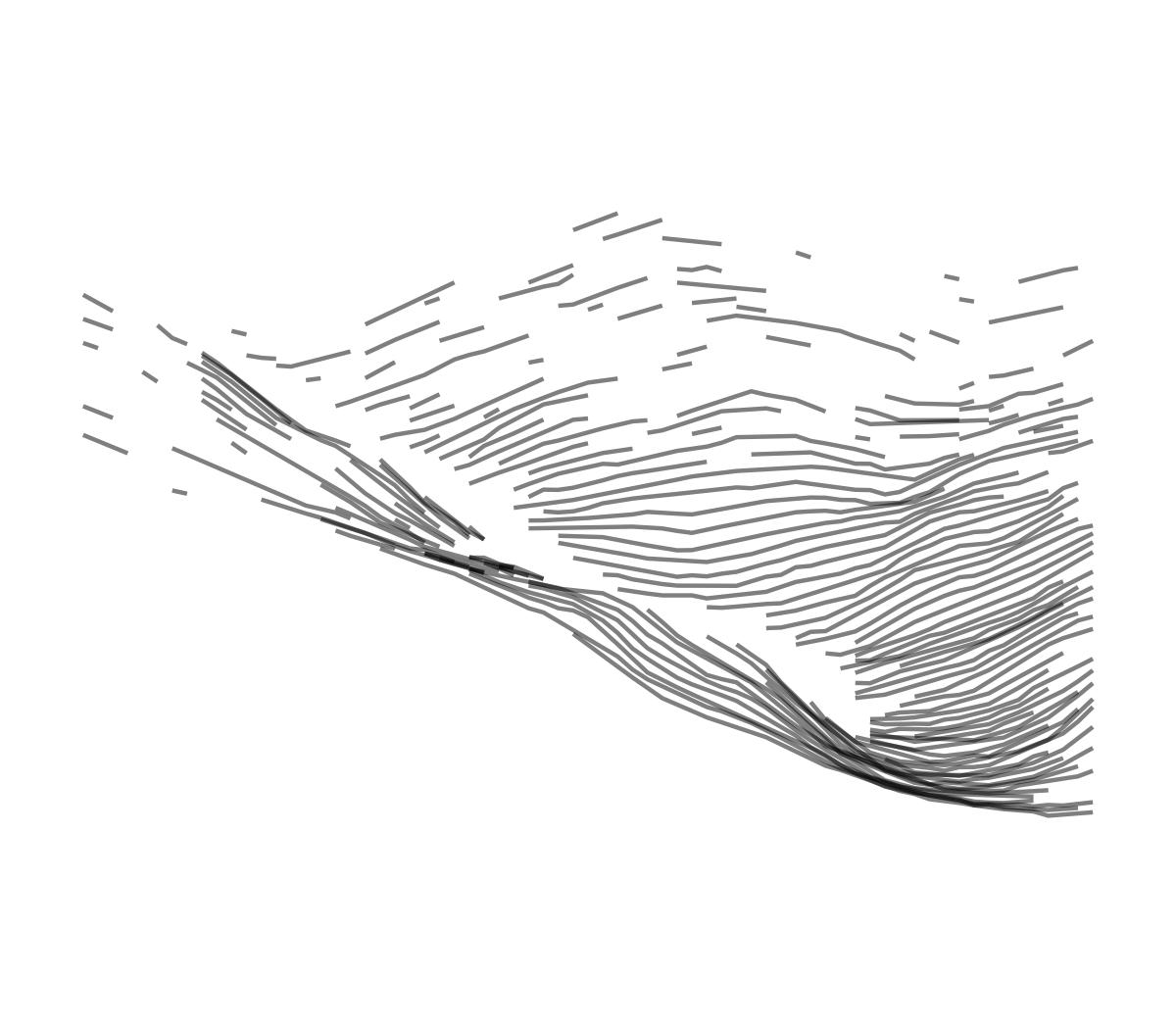 

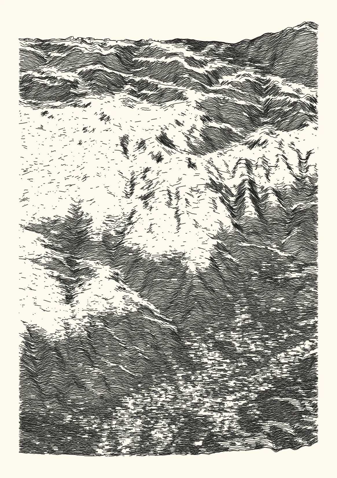
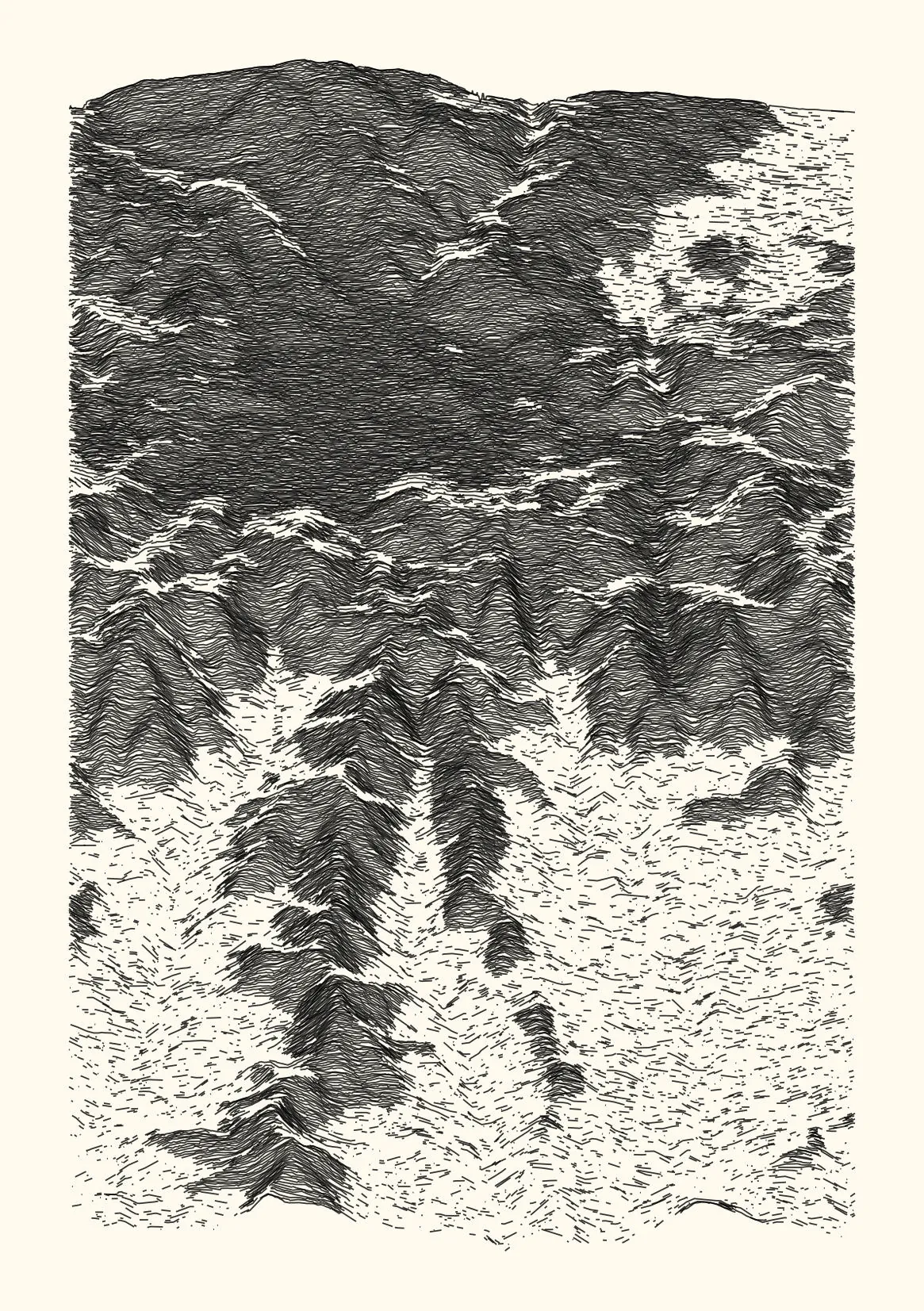
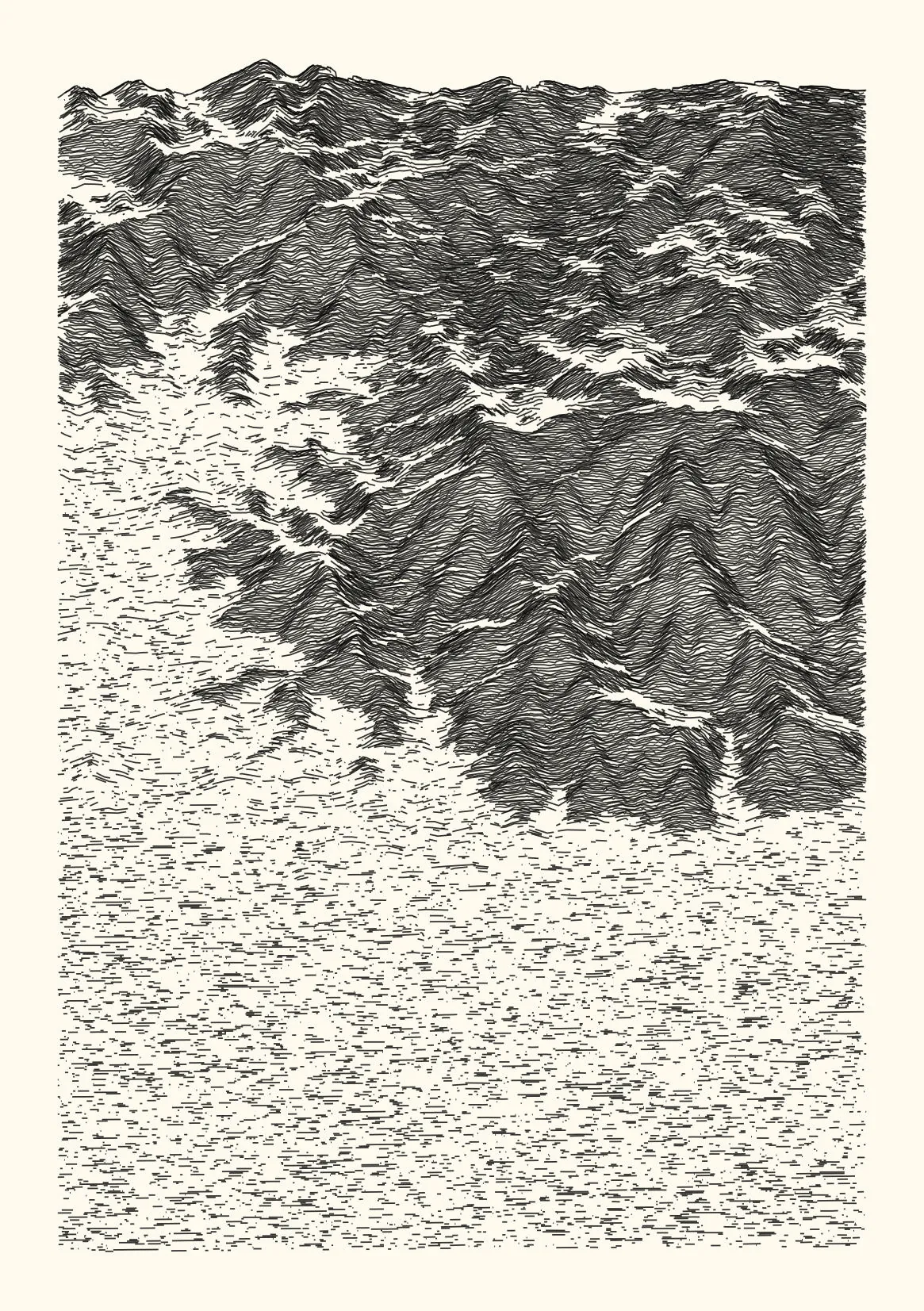
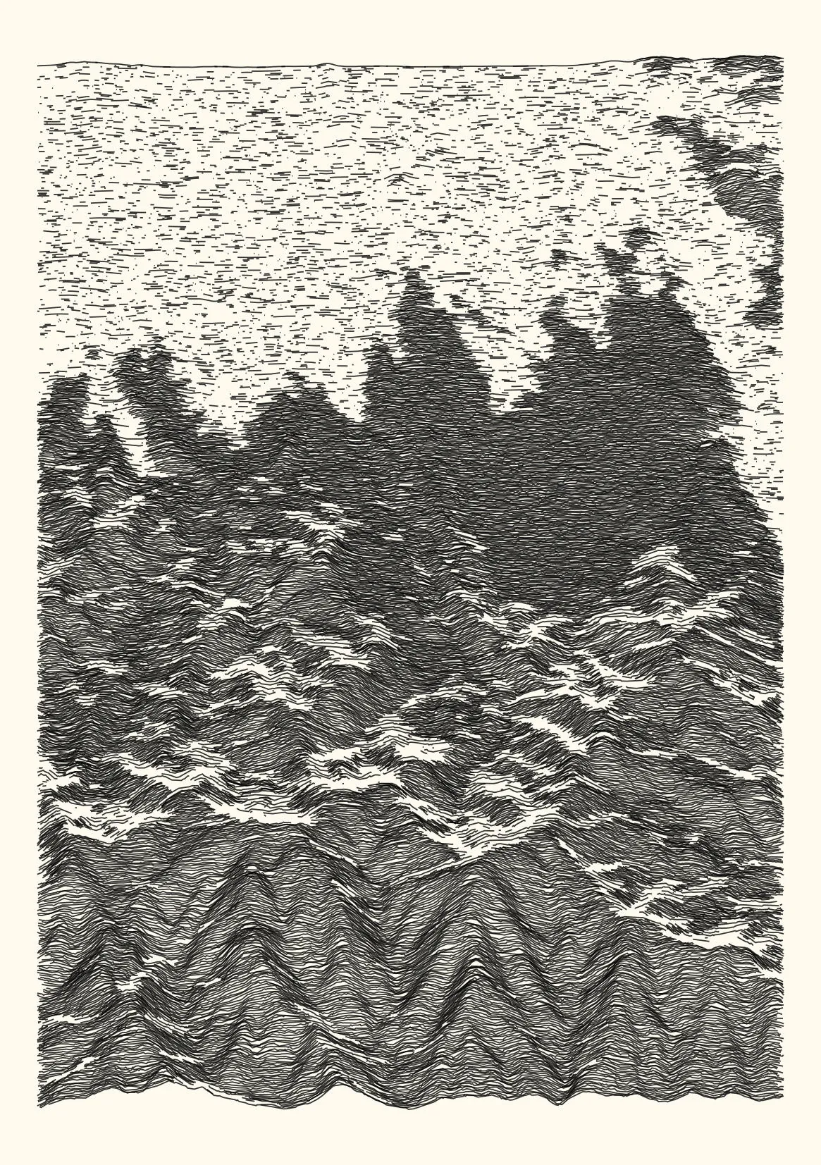
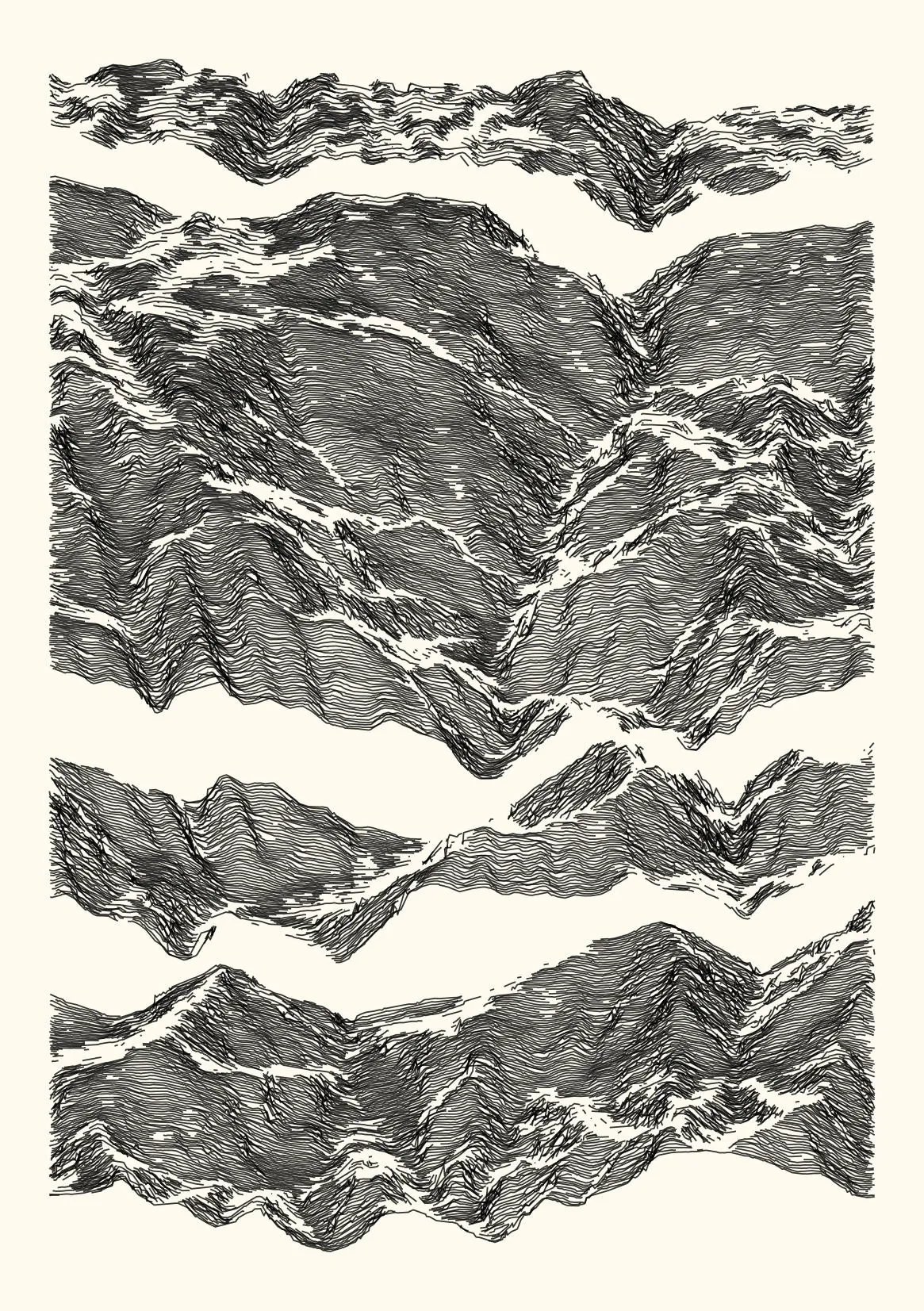
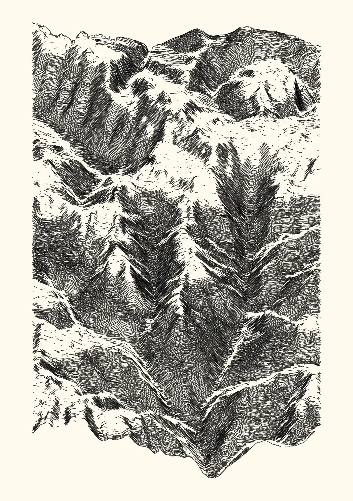
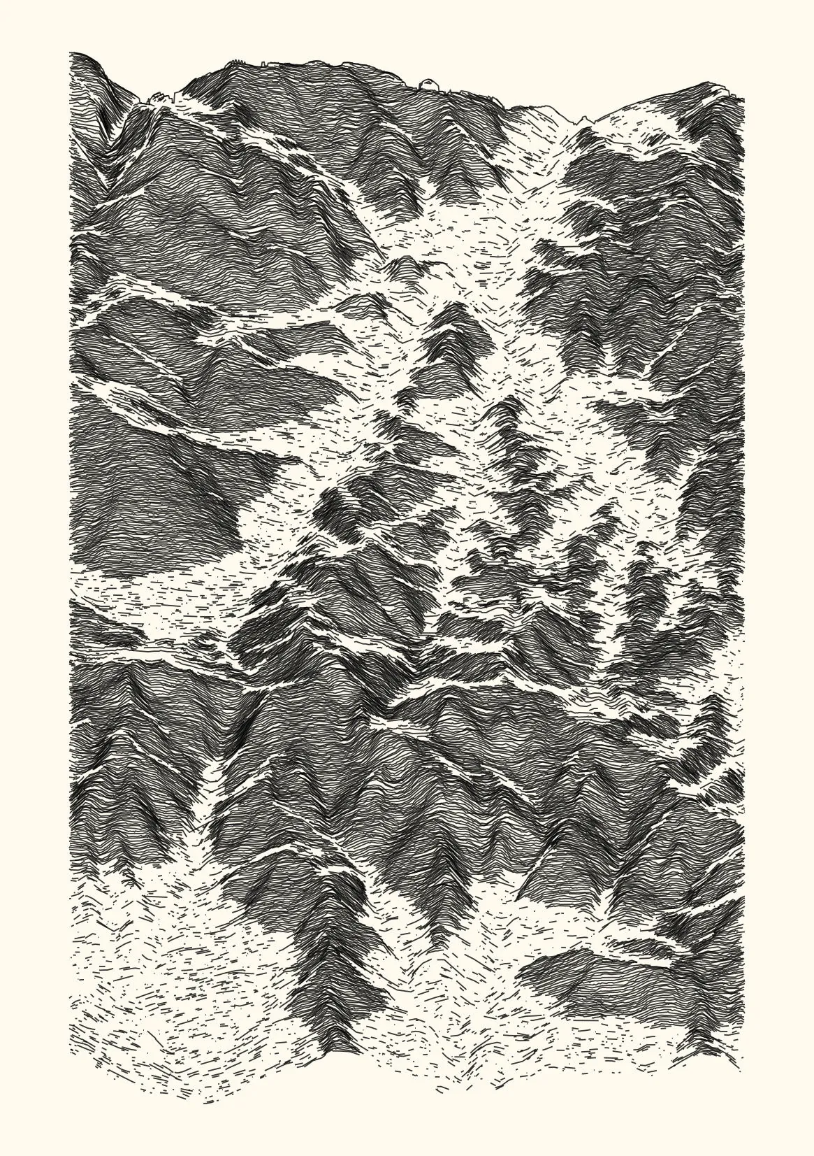
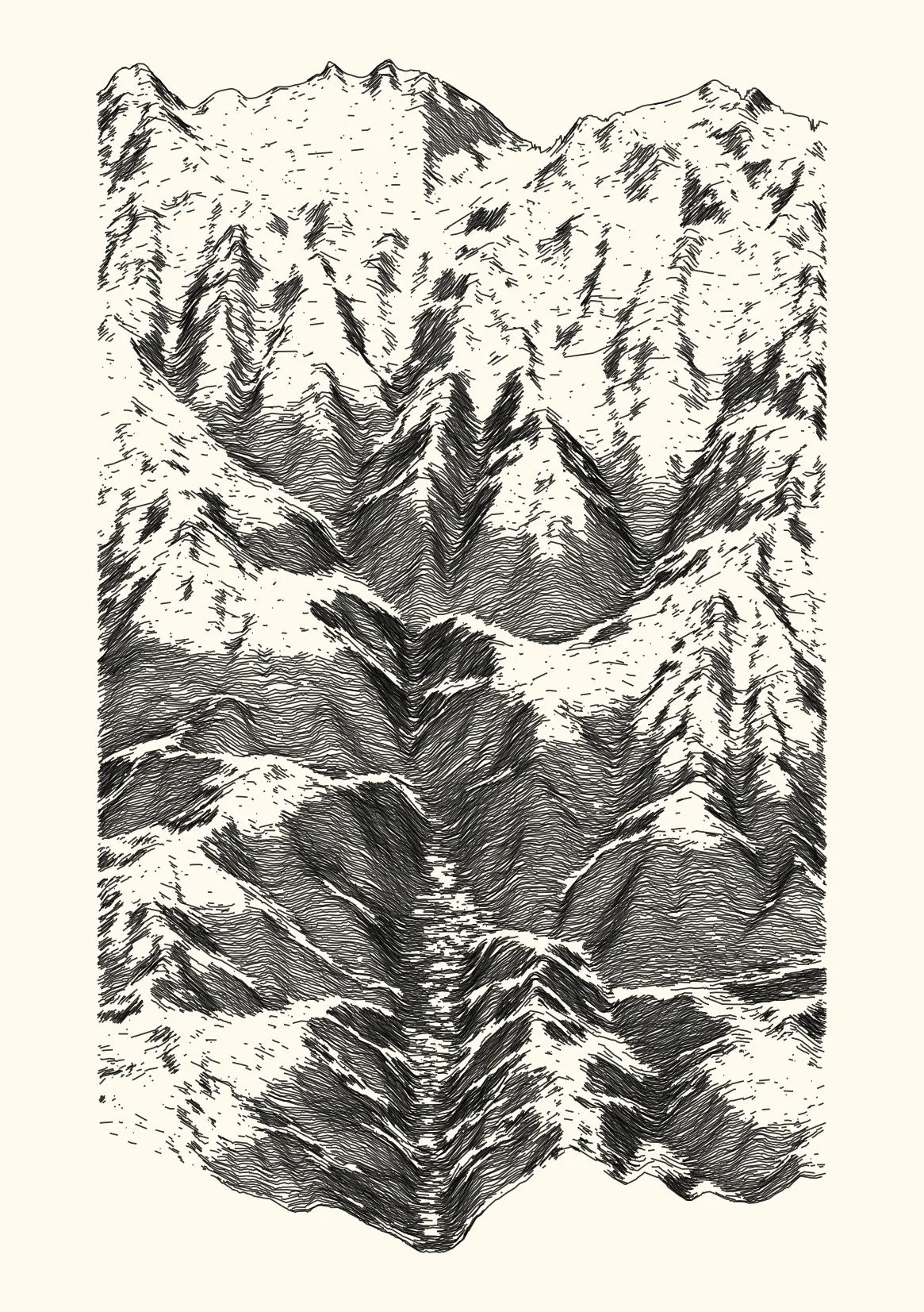
storm

Whole strips of lines are removed when the elevation variation is below a threshold. Additionally, an important jitter is added as a function of local slope value.

# functions

# scale the input vector with an exponential function
f_exp <- function(x, k = 1, a = 1, b = 0, scale = FALSE) {
  if (scale == TRUE) x = scales::rescale(x, to=c(0,1)) else x
  a * exp(k * x) + b
}

# find multiple non-consecutive minima in a vector (this is awful) 
get_extremum <- function(data, n = 5, w = 20, delta = 20, method = "max") {
  data |>
    mutate(
      y_smooth = RcppRoll::roll_mean(y_raw, n = w, na.rm = TRUE, fill = NA)
    ) |>
    filter((y_smooth - y_raw) > delta) |>
    filter(
      if_else(
        lag(y_raw, n = 1) > y_raw & lead(y_raw, n = 1) > y_raw,
        TRUE, FALSE)
    ) |>
    slice_min(y_raw, n = n)
}

# parameters
y_range = 5        # number of ridges to remove around selected ones
x_size = 5          # window of the rolling average 
z_remove = 0.5      # proportion of points to remove in lines
z_jitter = 4        # amount of jitter in elevation values


# get maximum number of ridgelines
n_ridge_max <- df_ridge |> distinct(y_rank) |> nrow()

# calculate local slope and remove points for flat areas
df_filter <- df_ridge |>
    group_by(y_rank) |> arrange(x_rank) |>
    mutate(
      z_slope = abs(
        (zn - lag(zn, default = 0)) / (xn - lag(xn, default = 0))
        ),
      z_slope = RcppRoll::roll_mean(z_slope, n = x_size, fill = NA_real_),
      zn = if_else(z_slope == 0, NA_real_, zn)
    ) |> ungroup()

# compute potential distortion on z-axis as a function of local slope on x-axis
# jitter by sampling in this distortion level for each point
df_sample <- df_filter |>
  group_by(y_rank) |>
  slice_sample(prop = (1 - z_remove)) |>
  mutate(z_jitter = f_exp(z_slope, k = 3.5, a = 0.3, scale = TRUE) * z_jitter) |>
  ungroup() |>
  mutate(
    z_jitter = runif(n(), -z_jitter, z_jitter),
    zn = zn + z_jitter
  )

# get ridges position with low elevation variance
index_strip <- df_sample |>
  group_by(y_rank) |>
  summarise(y_raw = sd(z, na.rm = TRUE)) |>
  get_extremum(n = as.integer(z_remove * 5), w = 30, delta = 3, method = "min") |>
  filter(between(y_rank, (y_range + 5), (n_ridge_max - y_range - 5)))

# remove strips of ridges based on previous index
df_plot <- anti_join(
  df_sample,
  df_sample |>
    distinct(y_rank) |>
    slice(
      index_strip |> pull(y_rank) |>
        map(~ (.x - y_range):(.x + y_range)) |>
        flatten_int()
    ),
  by = "y_rank"
)

# plot output
df_plot |> ggplot(aes(x, zn, group = y)) +
  geom_line(alpha = 0.5) + coord_fixed() + theme_void()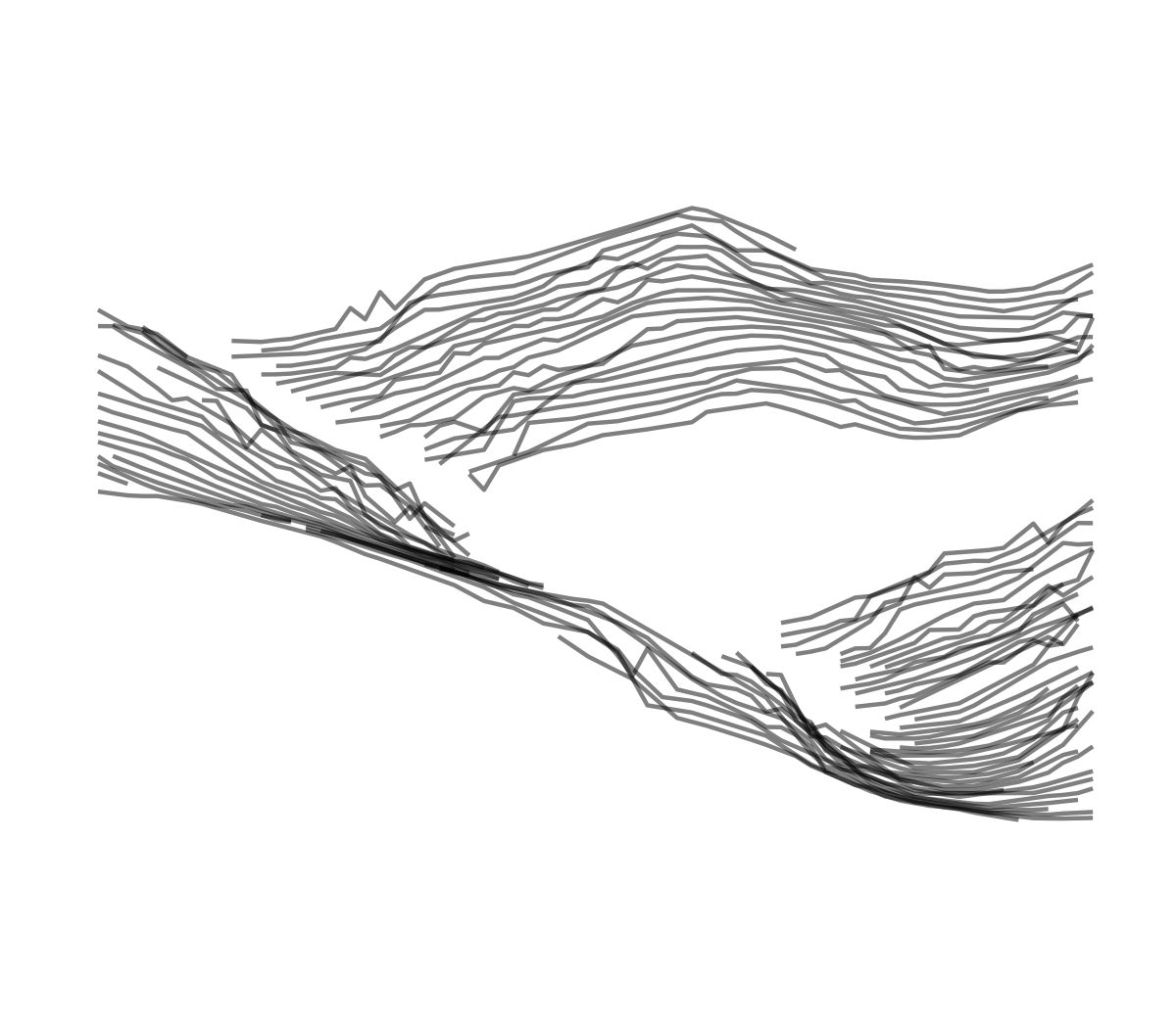 

Rendering

This step is essentially playing on opacity (either constant or variable along a line) and on the doubling of the line strokes to emulate pencil lines. Thanks to the R graphical devices, the same object can be exported to bitmap or vector files.

default

# parameters
z_remove = 0.5      # proportion of points to remove
z_jitter = 4        # amount of jitter in elevation values
p_alpha = 0.5       # mean opacity value

# randomly sample a proportion of points in a line, jitter their y-position.
df_plot <- df_ridge |>
  group_by(y_rank) |>
  slice_sample(prop = (1 - z_remove)) |>
  mutate(zn = jitter(zn, amount = z_jitter))

# render lines with a constant alpha value
df_plot |> ggplot(aes(x, zn, group = y)) +
  geom_line(alpha = p_alpha) + coord_fixed() + theme_void()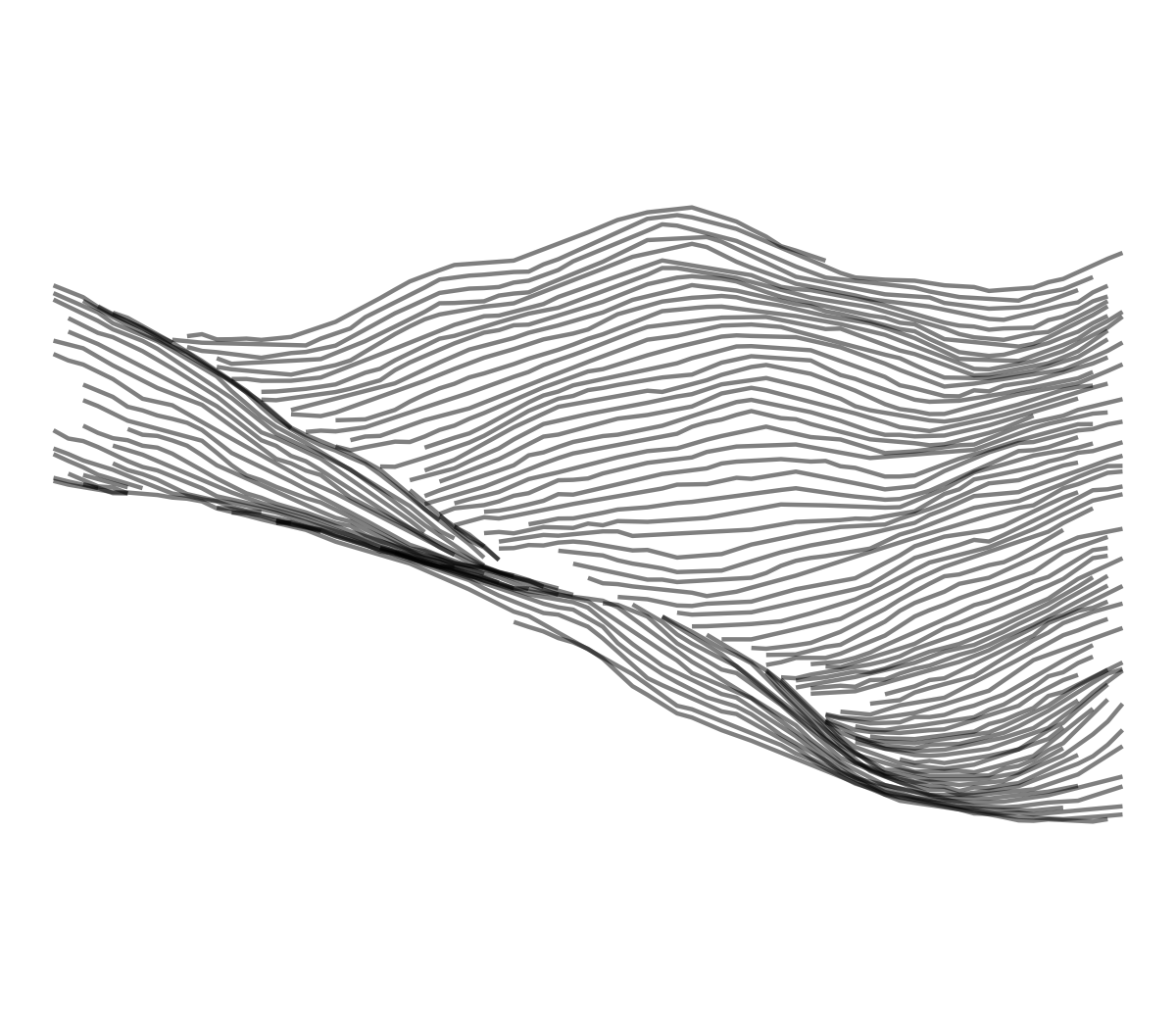 

variable opacity

# parameters
p_alpha_sd = 0.10   # dispersion of opacity value 

# render line with an alpha value sampled from a Gaussian distribution
df_plot |>
  mutate(z_alpha = rnorm(n(), p_alpha, p_alpha_sd)) |> 
  ggplot(aes(x, zn)) +
  geom_line(aes(group = y_rank, alpha = z_alpha)) +
  scale_alpha_identity() + coord_fixed() + theme_void()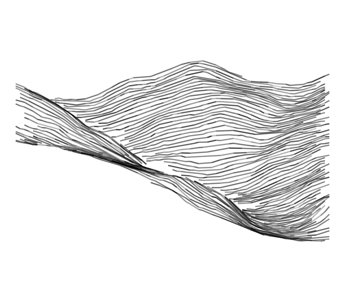 

variable opacity and double strokes

# functions
# fit a polynomial determined by one or more numerical predictors
f_loess <- function(data, span, n = 10) {

  # do not fit model if less than n non-na values
  if (sum(!is.na(data$zn)) < n) {

    return(rep(NA, nrow(data)))

  } else {

    m <- loess(zn ~ xn, data = data, na.action = na.exclude, span = span)
    return(predict(m))

  }
}

# parameters
p_span = 0.5      # span of the smoothing model (smaller fits the line)
p_length = 25     # minimal line length to apply the smoothing model

# render line with two strokes, and variable alpha
df_smooth <- df_plot |>
  group_by(y_rank) |> nest() |>
  mutate(z_smooth = map(data, ~ f_loess(., span = p_span, n = p_length))) |>
  unnest(c(data, z_smooth))

ggplot() +
  geom_line(
    data = df_plot |> mutate(z_alpha = rnorm(n(), p_alpha, p_alpha_sd)),
    aes(xn, zn, group = y_rank, alpha = z_alpha), na.rm = TRUE) +
  geom_line(
    data = df_smooth,
    aes(xn, z_smooth, group = y_rank), alpha = p_alpha) +
  scale_alpha_identity() + coord_fixed() + theme_void()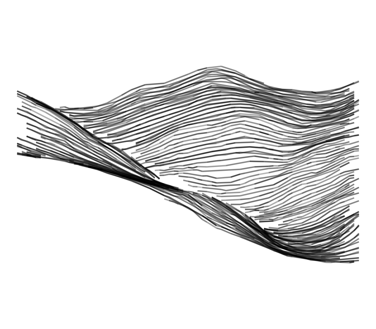

Iterations

These outputs were generated with the algorithm described previously, but based on a random location in the whole Pyrenees range (with a larger geographical area - 15x20 km, and a random cardinal orientation), and a random aesthetic style among the four presented ones. The algorithm can handle about 1000 iterations before repeating information (about 70 distinct 300 km2 regions with limited overlapping, 4 orientations, and 4 styles).

An example of 32 random iterations from this algorithm.